1随机变量的组合Combinations of random variables
X ± Y 的期望与方差Expected mean and variance for X ± Y
提醒Reminder
对任意两个随机变量 X 与 Y,有
而对两个相互独立的随机变量
独立正态随机变量的组合Combining independent normal random variables Y
若 X1 与 X2 是相互独立的正态随机变量,且
则 X1 + X2 与 X1 – X2 也都是正态随机变量:
Example:X1 and X2 are independent normal random variables
X1 ~ N(21, 12) and X2 ~ N(9, 6).
Find the expected mean and standard deviation of X1 – 2X2.
Solution:E[X1] =21, Var[X1] = 12 and E[X2] = 9, Var[X2] = 6
Example:The weights of empty coffee jars are normally distributed with mean 0.1 kg and standard deviation 0.02 kg. The weight of coffee in the jars is normally distributed with mean 1 kg and standard deviation 0.06kg.
Find the distribution of 12 full jars of coffee.
What is the probability that 12 full jars weigh more than 13⋅5 kg?
Solution:Let X1, X2, ... X12 be the weights of 12 empty jars and Y1, Y2, ... Y12 be the weights of coffee in the jars. X ~ N(0⋅1, 0⋅022) and Y ~ N(1, 0⋅062).
Let W be the total weight of 12 full jars then W = X1 + X2 + ... + X12 + Y1 + Y2 + ... + Y12.
Then E[W] = 12 E[X] + 12 E[Y] = 12 × 0⋅1 + 12 × 1 = 13⋅2
and, assuming independence,
Var[W] = 12 Var[X] + 12 Var[Y] = 12 × 0⋅022 + 12 × 0⋅062 = 0⋅048.
As we are combining normal distributions
the distribution for 12 full jars is N(13.2, 0⋅048). Answer
The probability that 12 full jars weigh more than 13⋅5 kg is
2抽样Sampling
数据收集方法Methods of collecting data
普查Taking a census
普查指观察总体中的每一个成员
它适用于以下情形
总体规模较小
或需要极高的精确度。
优点
能得到完全准确的结果,即完整的图景。
缺点
非常耗时且昂贵
当检验过程会破坏被测对象时无法使用
信息量太大,难以处理。
抽样Sampling
抽样指只观察或检验总体的一部分。
它更便宜,但得不到那么完整的图景。
样本的大小取决于所需的精确度(对于差异较大的总体,需要较大的样本才能达到合理的精度)。
简单随机抽样Simple random sampling
总体中的每个成员被选中的机会必须相等。
使用随机数表Using random number tables
要从 N 个抽样单元组成的总体中抽取容量为 n 的简单随机样本,先编制名单并给总体中的每个成员编号,然后用随机数表选取样本。
凡是超出总体编号范围的数字一律忽略 – 例如对编号 001 到 659 的总体使用三位随机数时,660 到 999 的数字都要跳过。
同一个数字第二次出现时也忽略。
优点
数字真正随机、不受偏倚影响
使用方便
每个成员被选中的机会已知且相等
缺点
样本容量较大时不适用。
抽签抽样
需要一份抽样框 – 即标出总体中的每个成员。把每个成员的姓名或编号写在一张票上(所有票的大小、颜色、形状都相同),把票全部放进容器中摇匀,然后不放回地抽票。
优点
票是随机抽出的。
使用方便。
每张票被抽中的机会已知(只要样本容量远小于票的总数,可视为常数)。
缺点
不适合大样本
需要抽样框。
系统抽样Systematic sampling
先编制一份有序名单,分成若干个大小相等、每组 50(或 n)的组。
再每隔 50(或 n)个从名单中抽取一名成员。
为确保名单上的第一个人不会被自动选中,必须用随机数表选出第一组中的成员,此后每隔 50(或 n)个抽取一名。
适用场合 总体过大、不适合简单随机抽样时。
优点
使用简单
适合大样本
缺点
只有在有序名单真正随机时才是随机的。
可能引入偏倚
分层抽样Stratified sampling
先把总体分成互不重叠(distinct)的组或层,然后抽取样本,使每一层在样本中所占的比例等于该层在总体中所占的比例。
Example:How would you take a stratified sample of 50 children from a school of 500 pupils divided as follows:
| Boys | Girls | |
|---|---|---|
| Upper sixth | 30 | 40 |
| Lower sixth | 30 | 30 |
| Fifth form | 70 | 60 |
| Fourth form | 60 | 70 |
| Third form | 50 | 60 |
Solution:As 50 is 1/10 of the total population, 1/10 of each stratum should be selected in the sample.
Thus the sample would comprise
| Boys | Girls | |
|---|---|---|
| Upper sixth | 3 | 4 |
| Lower sixth | 3 | 3 |
| Fifth form | 7 | 6 |
| Fourth form | 6 | 7 |
| Third form | 5 | 6 |
and simple random number sampling would be used within each stratum.
适用场合
样本较大
总体自然地分成互不重叠的组。
优点
在存在明显分层时,比简单随机抽样给出的估计更准确(或图景更具代表性)。
它能反映总体的结构。
缺点
层内的问题与任何简单随机样本相同
如果各层界定不清,层与层可能重叠。
有放回与不放回抽样Sampling with and without replacement
简单随机抽样是不放回抽样:总体中的每个成员最多被选中一次。
在有放回抽样中,总体中的每个成员可以被选中多于一次:这称为无限制随机抽样(unrestricted random sampling)。
配额抽样Quota sampling
这是一种非随机的方法。
先决定把总体分成哪些组,并确定每组要访问的人数,形成配额。
然后外出访问,把每个结果填入相应的配额。
如果有人拒绝回答,或属于已经填满的配额,就忽略此人的回答,继续访问,直到所有配额都填满。
适用场合 无法采用随机方法时 – 例如并不知道整个总体时(大城市中的无家可归者)。
优点
可以很快完成,因为用很小的样本就能得到有代表性的样本
成本降到最低
实施相当容易。
缺点
无法估计抽样误差(因为不是随机过程)
访问者可能把对象填进错误的配额
不回答的情况没有被记录
可能引入访问者偏倚
一手数据Primary data
一手数据是由将要使用这些数据的人、或代表其利益的人收集的数据。
优点
收集方法已知
精确度已知
收集到的正是所需的数据
缺点
在时间和精力上代价高
二手数据Secondary data
二手数据是并非由将要使用它的人、或代表其利益的人收集的数据。这类数据是现成的 – 例如政府的人口普查统计。
优点
获取成本低
可获得的数量大(例如互联网上)
很多数据逐年收集,可用来绘制趋势
缺点
收集方法可能未知
精确度可能未知
数据的格式可能难以处理
偏倚并不总能被识别。
3有偏与无偏估计量Biased & unbiased estimators
Example:A bag contains a large number of coins, of which 25 are 2p coins and 35 are 5p coins.
(a)X is the value of a single coin draw from the bag. Find the expected mean of all coins in the bag, µ = E[X].
Samples of size 3 are now drawn from the bag.
(b)Find the sampling distribution of X̅ and the expected value of (i) the median, and (ii) the mean.
(c)(i)The median, Q2, is used as an estimator of the mean of all the coins, µ. Show that Q2 is a biased estimator of µ, and find the bias.
(ii)The mean, X̅, is used as an estimator of the mean of all the coins, µ. Show that X̅ is an unbiased estimator of µ.
(d)kQ2 is now used as an unbiased estimator of the mean of all the coins. Find the value of k.
Solution:
(a)µ = E[X] = ∑xipi = 25 × 2 + 35 × 5 = 3∙8
(b)
| Sample | Probability | median | mean |
|---|---|---|---|
| (2,2,2) | (25)3 = 8125 | 2 | 2 |
| (2,2,5), (2,5,2), (5,2,2) | 3 × (25)2 × 35 = 36125 | 2 | 3 |
| (2,5,5), (5,2,5), (5,5,2) | 3 × 25 × (35)2 = 54125 | 5 | 4 |
| (5,5,5) | (35)3 = 27125 | 5 | 5 |
Sampling distribution
(i) Median
| Q2 = xi | pi | xipi |
|---|---|---|
| 2 | 8+36125 | 88125 |
| 5 | 54+27125 | 405125 |
| 493125 |
(ii) Mean
| X̅ = xi | pi | xipi |
|---|---|---|
| 2 | 8125 | 16125 |
| 3 | 36125 | 108125 |
| 4 | 54125 | 216125 |
| 5 | 27125 | 135125 |
| 475125 |
(c)(i)The median Q2 is used as the estimate of the mean.
From part (a) we know that the true value of the mean µ is 3⋅8, and in part (b) we have shown that E[Q2] = 3⋅944
and the bias is |E[Q2] – true value of µ| = |3⋅944 − 3⋅8| = 0⋅144
(ii) The mean X̅ is used as the estimate of the mean.
From part (a) we know that the true value of the mean µ is 3⋅8, and in part (b) we have shown that E[X̅] = 3⋅8
(d)If we now use kQ2 as an unbiased estimator of the mean value of all the coins.
If kQ2 is an unbiased estimator of µ, E[kQ2] = true value of µ
无偏估计量 Unbiased estimator:
若用 X(通常由样本求得)来估计总体参数 t 的值,则当 E[X] 等于参数 t 的真值时,X 是 t 的无偏估计量。
偏差 Bias:
若估计量 X 是有偏的,则偏差等于 E[X] 与参数 t 的真值之差。
Example:A sample of size 3 is drawn from a binomial distribution B(10, 0⋅25) and the mean, X̅, is calculated.
The probability of success, p, is estimated by p̂ = 110X. Show that p̂ is an unbiased estimator of p.
Solution:
For a sample {X1, X2, X3}, X̅ = 13(X1 + X2 + X3)
Example:A sample of size 4 is drawn from a continuous uniform distribution, U[3, β ]. The mean of the sample, X̅, is calculated.
The upper limit, β, is estimated by β̂ = 2X̅− 3. Show that β̂ is an unbiased estimator of β.
Solution:
For a sample {X1, X2, X3, X4}, X̅ = 14(X1 + X2 + X3 + X4)
which is the true value of the (unknown) upper limit, β.
关于有偏与无偏估计量的更多内容见附录。
µ 与 σ² 的无偏估计量Unbiased estimators of µ and σ2
从样本估计 µ 与 σ²Estimating µ and σ2 from a sample
我们通常并不知道总体的均值 µ 与方差 σ2。
为估计这些值,我们取一个容量为 n 的样本 {X1, X2, X3, …, Xn},并计算
样本均值,X̅ = 1n∑Xi,以及
这些可以与 S1 模块中总体方差的公式相对照。
可以证明 E[ X̅ ] = µ 的真值
⇒ X̅ = μ̂ 是总体均值 µ 的无偏估计量。
可以证明 E[(sd)x2] = n−1n σ 2 …… I
⇒ (sd)x2 是 σ² 的有偏估计量。
I ⇒ E[nn−1 (sd)x2] = nn−1 × n−1n σ 2 = σ 2,即方差的真值
⇒ nn−1 (sd)x2 = σ̂2 是总体方差 σ² 的无偏估计量。
(这些结果的证明见附录。)
注:Edexcel 课程同时用 S2 与 sx2 两个记号表示 σ² 的无偏估计。
另外,「样本方差」(Sample Variance)一词用来表示 σ² 的无偏估计,即总体的方差。
在本书中,我始终把方差 (sd)x2 理解为 1n∑Xi2 − X̅2 = 1n∑(X − X̅)2
要求 S2 或 sx2(σ² 的无偏估计量):–
先计算 (sd)x2,再乘以 nn−1
Example:
The weights of a sample of five chocolate bars produced by a machine were 56, 53, 57, 51 and 54 grams. Find unbiased estimators for the weight of all chocolate bars produced by that machine.
Solution:
| X | X − X̅ | (X − X̅)2 |
|---|---|---|
| 56 | 1⋅8 | 3⋅24 |
| 53 | -1⋅2 | 1⋅44 |
| 57 | 2⋅8 | 7⋅84 |
| 51 | -3⋅2 | 10⋅24 |
| 54 | -0⋅2 | 0⋅04 |
| 271 | 22⋅8 |
AnswerUnbiased estimators for the mean and variance of all chocolate bars are 54⋅2 grams and 5⋅7 grams2.
Example: The volume of water in each of a sample of 14 litre bottles of water from a day’s production is taken. The results are shown below, in ml.
1023, 1019, 1004, 1011, 1023, 1014, 1017, 1020, 1020, 1010, 1025, 1007, 1016, 1019
Find unbiased estimates for the mean and variance of all bottles produced on that day.
Solution:
First find the sample mean, X̅, = 1422814 = 1016⋅286….
(finding X − X̅ each time) would give unpleasant arithmetic,
so use (sd)x2 = 1n∑X2 − X̅2
∑X2 = 14460232
AnswerUnbiased estimators for the mean and variance of the whole day’s production are 1016⋅3 ml and 39⋅91 ml2.
Example: The weights of a sample of 15 packets of biscuits are recorded and give the following results.
Σ X = 3797 grams, and Σ X 2 = 973692.
Find unbiased estimators for the mean and variance of all biscuits produced by this process.
Solution: µ = X̅= 379715 = 253 ∙133 … = 252 ∙1 grams.
AnswerUnbiased estimators are μ̂ =252⋅1 g, and σ̂2 = 896⋅1 g2.
Example: The lengths of 10 rods are measured, and the sample has mean, X̅ = 26⋅7 cm and variance s2 = 76⋅9 cm2. An eleventh rod has length 30 cm.
Find (a) the mean and (b) the variance of the sample of 11 rods.
Solution: (a) With the sample mean there are no complications.
For n = 10, X̅10 = 11010∑i=1Xi = 26 ∙7 ⇒ 10∑i=1Xi = 267
For n = 11, 11∑i=1Xi = 267 + 30 = 297 ⇒ X11 = 11111∑i=1Xi = 29711 = 27 cm
(b)WARNING: The question refers to the variance of the sample, which means the unbiased estimate of the variance of the population.
For 11 rods, sample mean is 27 cm, and sample variance is 70⋅2 cm2.
4置信区间与显著性检验Confidence intervals and significance tests
样本均值的抽样分布Sampling distribution of the mean
设 X 为从均值为 µ、标准差为 σ 的总体中抽取的随机变量。
若 {X1, X2, … , Xn} 是容量为 n 的随机样本,其均值为 X̅ = X1 + X2 + ... + Xnn,则对 i = 1, 2, 3, …, n 有 E[Xi] = µ,且 Var[Xi] = σ2。
由此,样本均值所构成的总体的期望均值为
而样本均值所构成的总体的期望方差为
这说明:若抽取非常多个样本并算出每个样本的均值,则这些均值的均值将为 µ,而这些均值的方差将为 σ2n。
还可以证明,只要 n 足够大,样本均值就构成正态分布。
于是可以说:对于从均值为 µ、方差为 σ2 的总体中抽取的样本,均值的抽样分布为 N(µ, σ2n)。
中心极限定理与标准误Central limit theorem and standard error
中心极限定理 the central limit theorem 指出:
若 {X1, X2, …, Xn} 是容量为 n 的随机样本,取自任意均值为 µ、方差为 σ2 的总体,则样本均值的总体
(i)的期望均值为 µ
(ii)的期望方差为 σ2n
(iii)当 n 足够大时构成正态分布。
即
当样本容量很大(约 > 50)时,抽样就要用中心极限定理 —— 此时无论原总体是什么分布,样本均值的总体都近似正态。
样本均值的标准误为 σ√n。
Example:A sample of size 50 is taken from a population of eggs with mean 23⋅4 grams and variance 36 grams2.
(i)Find the probability that a single egg weighs more than 25 grams.
(ii)Find the probability that the sample mean is larger than 25.
(iii)What assumptions did you make?
Solution:
(i)The weight of a single egg, X ∼ N(23⋅4, 62)
(ii)µ = 23⋅4, σ2 = 36
The sample mean X̅ ∼ N(23⋅4, ( 6√50 )2)
= 1 – Φ(1⋅89) = 1 – 0⋅9706 (from Normal tables)
= 0 ⋅0294.
(iii)We have assumed the Central Limit Theorem: in particular that the sample means form a normal distribution.
置信区间Confidence intervals
中心极限定理示例Central Limit Theorem Example
Example:A biscuit manufacturer makes packets of biscuits with a nominal weight of 250 grams. It is known that over a long period the variance of the weights of the packets of biscuits produced is 25 grams2. A sample of 10 packets is taken and found to have a mean weight of 253⋅4 grams. Find 95% confidence limits for the mean weight of all packets produced by the machine.
Solution:
First assume that the machine is still producing packets with the same variance, 25.
Suppose that the mean weight of all packets of biscuits is µ grams then the population of all packets has mean µ and standard deviation 5.
From the central limit theorem we can assume that the sample means form an approximately normal population with mean µ and standard error (standard deviation) σ√n = 5√10 = 1⋅5811
95% of the samples will have a mean in the region
We assume that the mean of this sample, 253⋅4, lies in this region
This means that 95% of the samples will give an interval which contains the mean
and we say that [250⋅3 g, 256⋅5 g] is a 95% confidence interval for µ.
This means that there is a 0⋅95 probability that this interval contains the true mean.
It does not mean that there is a probability of 0⋅95 that the true mean lies in this interval - the true mean is a fixed number, and either does or does not lie in the interval so the probability that the true mean lies in the interval is either 1 or 0.
实际计算时,我们直接跳到例题的最后一行:
因为 P(Z –1⋅9600 < z < 1⋅9600) = 0⋅95 查表得 P(Z > 1⋅9600) = 0⋅025
因为 P(Z –1⋅6449 < z < 1⋅6449) = 0⋅90 查表得 P(Z > 1⋅6449) = 0⋅05
其他置信水平可由正态分布表查出对应的 z 值。
Example:A sample of 64 packets of cornflakes has a mean weight X̅ = 510 grams and a variance S2 = 36 grams2. Find 90% confidence limits for the mean weight of all packets.
(Note that the ‘sample variance’ is taken as the unbiased estimate of µ2.)
Solution:
We assume that the sample variance = the variance of the population of all packets
Now find standard deviation (standard error) of the sampling distribution of the mean (population of sample means),
For 90% confidence limits z = ± 1⋅6449 (remember to use the 4 D.P. tables after the Normal Dist. tables),
using the sample mean X̅ = 510 grams
Note that we have assumed that the unbiased estimate, S2 (=36), is the actual variance, µ2, of the population.
This is a reasonable assumption as the number in the sample, 64, is large and the error introduced is therefore small.
显著性检验——总体方差已知Significance testing – variance of population known
正态分布的均值Mean of normal distribution
Example:A machine, when correctly set, is known to produce ball bearings with a mean weight of 84 grams with a standard deviation of 5 grams. The production manager decides to test whether the machine is working correctly and takes a sample of 120 ball bearings. The sample has mean weight 83.2 grams. Would you advise the production manager to alter the setting of his machine? Use a 5% significance level.
Solution:
1)H0: µ = 84 grams
2)H1: µ ≠ 84 grams⇒ 2 tail test
(Note that the machine is not working correctly if the test result is too high or too low)
3)5% Significance level
4)The Test
We assume that the machine is still working with a standard deviation of σ = 5 g.
From H0, the mean weight of all ball bearings is assumed to be µ = 84 g.
These are the parameters for the population of all ball bearings.
We want to test a sample mean and therefore need the mean and standard deviation of the population of sample means (the sampling distribution of the sample mean, X̅).
and
We have an observed mean of 83⋅2
For a two-tailed test at 5%, we take 2⋅5% at
each end
= (1 – Φ(1⋅75)) = 0⋅0401
= 4⋅01% > 2⋅5%
and so not significant at the 5% level.
5)Conclusion
Do not reject H0 at the 5% level and advise the production manager that there is evidence that he should not change his setting, or that there is evidence that the machine is working correctly, etc.
两个正态分布均值之差Difference between means of normal distributions
设 X 与 Y 是来自不同正态分布的两个相互独立的随机变量 —— X ∼ N(µx, σx2) 与 Y ∼ N(µy, σy2)。
若从这两总体分别抽取容量为 nx 与 ny 的样本,则样本均值的分布 X̅ 与 Y̅ 都是正态的
Example:The weights of chocolate bars produced by two machines, A and B, are known to be normally distributed with variances σA2 = 4 and σB2 = 3 grams2. Samples are taken from each machine of sizes nA = 25 and nB = 16 which have means X̅A = 123⋅1 and X̅B = 124⋅4 grams. Is there any evidence at the 5% significance level that the bars produced by machine B are heavier than the bars produced by machine A?
Solution:
Suppose that the mean weights for all bars from the two machines are µA and µB
H0:µA = µB
H1:µB > µA one-tail test at 5% level
The test statistic is the observed difference between sample means, X̅B − X̅A = 124⋅4 – 123⋅1 = 1⋅3,
and we must find the variance of this population of differences of sample means (the sampling distribution of differences of sample means).
Consider the population of differences of sample means X̅B − X̅A.
Firstly, for the population of sample means for machine B
and secondly, for the population of sample means for machine A
and so for the population of differences of sample means
The observed difference, the test statistic, is 124⋅4 – 123⋅1 = 1⋅3
The Central Limit Theorem tells us that we have a Normal distribution
= 1 – Φ(2⋅2053)
= 1 – Φ(2⋅20) = 1 – 0⋅9861 = 0⋅0134
= 1⋅34% < 5%
Fortunately (!) the formula for testing the difference between sample means
is in your formula booklet.
显著性检验——总体方差未知、大样本Significance testing – variance of population NOT known, large sample
当总体方差 µ 2 未知、而样本又是大样本时,我们假定样本的方差(即 µ2 的无偏估计)S2 就是总体方差 µ2。
由于样本很大,由此引入的误差很小。
正态分布的均值Mean of normal distribution
Example:A machine usually produces steel rods with a mean length of 25⋅4 cm. The production manager wants to test 80 rods to see whether the machine is working correctly. The sample has mean 25⋅31 cm and variance 0⋅332 cm2. Advise the production manager, using a 5% level of significance.
Solution:
H0:µ = 25⋅4.
H1:µ≠ 25⋅4 two-tail test, 2⋅5% in each tail
We assume that population variance σ2 = the sample variance S2 = 0⋅332
For the population of sample means (the sampling distribution of the sample means)
and
The observed sample mean is 25.31 and for a two-tail test at 5% we consider
重要假设Important assumption
样本方差 S2 取作 σ̂2,即总体方差 µ2 的无偏估计;随后我们假定总体方差等于该无偏估计。
均值之差Difference between means
Example:A firm has two machines, A and B, which make steel cable. 40 cables produced by machine A have a mean breaking strain of 1728 N and variance of 752 N2, whereas 65 cables produced by machine B have a mean breaking strain of 1757 N and a variance of 632 N2. Is there any evidence, at the 10% level, to suggest that machine B is producing stronger cables than machine A?
Solution:
Let µA and µB be the mean breaking strengths of all cables produced by machines A and B.
1)H0:µA = µB
2)H1:µB > µA 1 tail test
3)Significance Level 10%.
4)The Test
For Machine A
We assume that the population variance, σA2 = the sample variance, SA2 = 752
For Machine B
We assume that the population variance, σB2 = the sample variance, SB2 = 632
For differences in sample means X̅B − X̅A
We have an observed difference in means,
test statistic, X̅B − X̅A = 1757 – 1728 = 29
and for a 1-tail test that B is stronger
we need the area to the right of 29 mean is treated as continuous, so do not use 28.5
which is significant at 10%.
5)Conclusion
Reject H0 at the 10% level and conclude that there is evidence that machine B produces cables with a greater mean strength than machine A.
5拟合优度与 χ2 检验Goodness of fit, χ2 test
一般要点General points
❑ χ2 检验只能用于检验两组频数 – 观测频数,以及由假设计算出的期望频数。
❑ 期望频数不必是整数(保留 2 位小数)。
❑ χ2 = ∑ (Oi − Ei)2Ei,其中 Oi 与 Ei 分别为观测频数与期望频数。
❑ 若某一组的期望频数小于 5,则必须把这一组与下一组(或下两组)合并。
❑ 自由度 ν 等于(必要时合并后的)格子数减去连接这些频数的线性方程个数。
离散均匀分布Discrete uniform distribution
Example:A die is rolled 300 times and the frequency of each score recorded.
| Score: | 1 | 2 | 3 | 4 | 5 | 6 |
| Frequency: | 43 | 49 | 54 | 57 | 46 | 51 |
Test whether the die is fair at the 2⋅5% level of significance.
Solution:
H0:The die is fair, the probability of each score is 1/6.
H1:The die is not fair, the probability of each score is not 1/6.
The expected frequencies are all 1/6× 300 = 50 and we have
| Observed frequency | Expected frequency | (Oi − Ei)2Ei | |
| 1 | 43 | 50 | 0⋅98 |
| 2 | 49 | 50 | 0⋅02 |
| 3 | 54 | 50 | 0⋅32 |
| 4 | 57 | 50 | 0⋅98 |
| 5 | 46 | 50 | 0⋅32 |
| 6 | 51 | 50 | 0⋅02 |
| Totals | 300 | 300 | 2⋅64 |
and ν = number of degrees of freedom = n – 1 = 6 – 1 = 5
since the total is a linear equation connecting the frequencies and is fixed.
From tables we see that χ25(2⋅5%) = 12⋅832 > 2⋅64 , so our observed result is not significant.
We do not reject H0 and conclude that the die is fair.
连续均匀分布Continuous uniform distribution
这与离散均匀分布非常相似,但要留意组界并求出期望频数。
二项分布Binomial distribution
对于 H0:二项分布 B(30, 0⋅3) 拟合良好,我们用观测频数的均值来计算期望频数,因此 Oi 与 Ei 给出相同的均值与总和:于是有 2 个线性方程连接这些频数,故 ν = n – 2。
但 H0:二项分布 B(30, 0⋅3) 拟合良好时,用 Oi 与 Ei 得到的均值会不同:于是只有 1 个线性方程(总和)连接这些频数,故 ν = n – 1。
泊松分布Poisson distribution
对于 H0:泊松分布拟合良好,我们用观测频数的均值来计算期望频数,因此 Oi 与 Ei 给出相同的均值与总和:于是有 2 个线性方程连接这些频数,故 ν = n – 2。
但 H0:泊松分布 P0(3) 拟合良好时,用 Oi 与 Ei 得到的均值会不同:于是只有 1 个线性方程(总和)连接这些频数,故 ν = n – 1。
Example:A switchboard operator records the number of new calls in 69 consecutive one-minute periods in the table below.
| number of calls | 0 | 1 | 2 | 3 | 4 | 5 | ≥ 6 |
| frequency | 6 | 9 | 11 | 15 | 13 | 9 | 6 |
a)Say why you think that a Poisson distribution might be suitable.
b)Find the mean and variance of this distribution. Do these figures support the view that they might form a Poisson distribution?
c)Test the goodness of fit of a Poisson distribution at the 5% level.
Solution:
a)Telephone calls are likely to occur singly, randomly, independently and uniformly which are the conditions for a Poisson distribution.
b)Treating ≥ 6 as 7 we calculate the mean and variance
| x | f | xf | x2f |
| 0 | 6 | 0 | 0 |
| 1 | 9 | 9 | 9 |
| 2 | 11 | 22 | 44 |
| 3 | 15 | 45 | 135 |
| 4 | 13 | 52 | 208 |
| 5 | 9 | 45 | 225 |
| 7 | 6 | 42 | 294 |
| 69 | 215 | 915 |
From these figures we can see that the mean and variance are approximately equal: since the mean and variance of a Poisson distribution are equal this confirms the view that the distribution could be Poisson.
c)H0:The Poisson distribution is a suitable model
H1: The Poisson distribution is not a suitable model.
The Poisson probabilities can be calculated from P(r) = λre−λr! where λ = 3⋅12, and the expected frequencies by multiplying by N = 69.
Note that the probability for ≥ 6 is found by adding the other probabilities and subtracting from 1.
| x | O | p | E | O (grouped) | E (grouped) | (O − E)2E |
| 0 | 6 | 0⋅044337 | 3⋅059234 | |||
| 1 | 9 | 0⋅138151 | 9⋅532395 | 15 | 12⋅59 | 0⋅461326 |
| 2 | 11 | 0⋅215235 | 14⋅8512 | 11 | 14⋅85 | 0⋅998148 |
| 3 | 15 | 0⋅223553 | 15⋅42515 | 15 | 15⋅43 | 0⋅011983 |
| 4 | 13 | 0⋅174145 | 12⋅01597 | 13 | 12⋅02 | 0⋅079900 |
| 5 | 9 | 0⋅108525 | 7⋅488214 | 9 | 7⋅49 | 0⋅304419 |
| ≥ 6 | 6 | 0⋅096056 | 6⋅627836 | 6 | 6⋅63 | 0⋅059864 |
| 69 | 69 | 69.01 | 1.915641 |
The expected frequency for x = 0 is 3.06 < 5 so it has been grouped with x = 1.
Thus we have n = 6 classes (after grouping) and ν = n – 2 = 4
We have calculated χ2 = 1.92 < 9.488 which is not significant so we do not reject H0
and conclude that the Poisson distribution is a suitable model.
正态分布The normal distribution
对于 H0:正态分布拟合良好,我们用观测频数的均值与方差来计算期望频数,因此 Oi 与 Ei 给出相同的均值、方差与总和:于是有 3 个线性方程连接这些频数,故 ν = n – 3。
但 H0:正态分布 N(14, 32) 拟合良好时,用 Oi 与 Ei 得到的均值与方差会不同:于是只有 1 个线性方程(总和)连接这些频数,故 ν = n – 1。
Example:The sizes of men’s shoes purchased from a shoe shop in one week are recorded below.
| size of shoe | ≤ 6 | 7 | 8 | 9 | 10 | 11 | ≥ 12 |
| number of pairs | 14 | 19 | 29 | 45 | 40 | 21 | 7 |
Is the manager’s assumption that the normal distribution is a suitable model justified at the 5% level?
Solution:
H0:The normal distribution is a suitable model
H1:The normal distribution is not a suitable model.
The total number of pairs, mean and standard deviation are calculated to be 175, 8.886 and 1.713 (taking ≤ 6 as 5 and ≥ 12 as 12)
Remembering that size 8 means from 7.5 to 8.5 we need to find the area between 7.5 and 8.5 and multiply by 175 to find the expected frequency for size 8, and similarly for other sizes.
| x | z = x − ms | Φ(z) | class | area = p | E = 175p | O | (O − E)2E |
| 6.5 | -1.39 | 0.082 | < 6.5 | 0.082 | 14.4 | 14 | 0.01 |
| 7.5 | -0.81 | 0.209 | 6.5 to 7.5 | 0.209 – 0.082 = 0.127 | 22.2 | 19 | 0.46 |
| 8.5 | -0.23 | 0.409 | 7.5 to 8.5 | 0.409 – 0.209 = 0.200 | 35.0 | 29 | 1.03 |
| 9.5 | 0.36 | 0.641 | 8.5 to 9.5 | 0.641 – 0.409 = 0.232 | 40.6 | 45 | 0.48 |
| 10.5 | 0.94 | 0.826 | 9.5 to 10.5 | 0.826 – 0.641 = 0.185 | 32.4 | 40 | 1.78 |
| 11.5 | 1.53 | 0.937 | 10.5 to 11.5 | 0.937 – 0.826 = 0.111 | 19.4 | 21 | 0.13 |
| > 11.5 | 1 – 0.937 = 0.063 | 11.0 | 7 | 1.45 | |||
| 5.34 |
n = 7 classes & 3 linear equations connecting the frequencies (N, m ,s) ⇒ν = n – 3 = 4.
χ24(5%) = 9.488 and we have calculated χ2 = 5.34 < 9.488 and so we do not reject H0 and therefore conclude that the normal distribution is a suitable model.
列联表Contingency tables
对于一个 5 × 4 表,若每行与每列的总和都固定,则 ‘?’ 格代表自由度,因为只要知道这 ? 个值,其余格子里的频数就可以算出来。
| A | B | C | D | E | 合计 | |
| W | ? | ? | ? | ? | ✓ | |
| X | ? | ? | ? | ? | ✓ | |
| Y | ? | ? | ? | ? | ✓ | |
| Z | ✓ | |||||
| 合计 | ✓ | ✓ | ✓ | ✓ | ✓ | ✓ |
因此共有 (5 – 1) × (4 – 1) = 12 个。
推广之,对于 m×n 表,自由度为 (m – 1)(n – 1)。
Example:Natives of England, Africa and China were classified according to blood group giving the following table.
| O | A | B | AB | |
| English | 235 | 212 | 79 | 83 |
| African | 147 | 106 | 30 | 51 |
| Chinese | 162 | 135 | 52 | 43 |
Is there any evidence at the 5% level that there is a connection between blood group and nationality?
Solution:
H0:There is no connection between blood group and nationality.
H1:There is a connection between blood group and nationality.
First redraw the table showing totals of each row and column
| O | A | B | AB | totals | |
| English | 235 | 212 | 79 | 83 | 609 |
| African | 147 | 106 | 30 | 51 | 334 |
| Chinese | 162 | 135 | 52 | 43 | 392 |
| totals | 544 | 453 | 161 | 177 | 1335 |
Now we need to calculate the expected frequency for English and group O. There are 609 English and 1335 people altogether so 609/1335 of the people are English, and from H0 we know that there is no connection between blood group and nationality, so there should be 609/1335 of those with group O who are also English
this can become automatic if you notice that you just multiply the totals for the row and column concerned and divide by the total number
| O | A | B | AB | totals | |
| English | 609 × 5441335 = 248.2 | 609 × 4531335 = 206.6 | 609 × 1611335 = 73.4 | 609 × 1771335 = 80.7 | 608.9 |
| African | 334 × 5441335 = 136.1 | 334 × 4531335 = 113.3 | 334 × 1611335 = 40.3 | 334 × 1771335 = 44.3 | 334 |
| Chinese | 392 × 5441335 = 159.7 | 392 × 4531335 = 133.0 | 392 × 1611335 = 47.3 | 392 × 1771335 = 52.0 | 392 |
| totals | 544 | 452.9 | 161 | 177 | 1335 |
The value of χ2 is calculated below
| Observed frequency | Expected frequency | (O − E)2E |
| 235 | 248.2 | 0.70 |
| 212 | 206.6 | 0.14 |
| 79 | 73.4 | 0.43 |
| 83 | 80.7 | 0.07 |
| 147 | 136.1 | 0.87 |
| 106 | 113.3 | 0.47 |
| 30 | 40.3 | 2.63 |
| 51 | 44.3 | 1.01 |
| 162 | 159.7 | 0.03 |
| 135 | 133.0 | 0.03 |
| 52 | 47.3 | 0.47 |
| 43 | 52.0 | 1.56 |
| 8.41 |
We have ν = (4 – 1)(3 – 1) = 6 degrees of freedom and χ26(5%) = 12.592 .
We have calculated χ2 = 8.41 < 12.592
⇒ do not reject H0 and therefore conclude that there is no connection between nationality and blood group.
6回归与相关Regression and correlation
斯皮尔曼等级相关系数Spearman’s rank correlation coefficient
排名与并列名次Ranking and equal ranks
排名就是把一组数字按大小顺序排列,并给每一个数指定它的位置,即名次。
若几个数相等,则取它们在「互不相同」时本应得到的那些名次的平均值作为它们共同的名次。
Example:Rank the following numbers: 45, 65, 76, 56, 34, 45, 23, 67, 65, 45, 81, 32.
Solution:First put in order and give ranks as if all were different: then give the average rank for those which are equal.
| Numbers: | 81 | 76 | 67 | 65 | 65 | 56 | 45 | 45 | 45 | 34 | 32 | 23 |
| Actual rank | 1 | 2 | 3 | 4= | 4= | 6 | 7= | 7= | 7= | 10 | 11 | 12 |
| Rank (if all different) | 1 | 2 | 3 | 4 | 5 | 6 | 7 | 8 | 9 | 10 | 11 | 12 |
| average for equal ranks | 4+52 = 412 | 7+8+93 = 8 | ||||||||||
| Modified rank | 1 | 2 | 3 | 4½ | 4½ | 6 | 8 | 8 | 8 | 10 | 11 | 12 |
You must now calculate the PMCC, not Spearman, using the modified ranks.
斯皮尔曼等级相关系数Spearman’s rank correlation coefficient
要比较同一组 n 个对象的两种排名,先求出每一对名次之差 d,然后计算斯皮尔曼等级相关系数
它与这两组名次的积矩相关系数相同,因此可知
Example:Ten varieties of coffee labelled A, B, C, ..., J were tasted by a man and a woman. Each ranked the coffees from best to worst as shown.
| Man: | G | H | C | D | A | E | B | J | I | F |
| Woman: | C | B | H | G | J | D | I | E | F | A |
Find Spearman’s rank correlation coefficient.
Solution:Rank for each person, find d and then rs.
| Coffee | Man | Woman | d | d2 |
| A | 5 | 10 | -5 | 25 |
| B | 7 | 2 | 5 | 25 |
| C | 3 | 1 | 2 | 4 |
| D | 4 | 6 | -2 | 4 |
| E | 6 | 8 | -2 | 4 |
| F | 10 | 9 | 1 | 1 |
| G | 1 | 4 | -3 | 9 |
| H | 2 | 3 | -1 | 1 |
| I | 9 | 7 | 2 | 4 |
| J | 8 | 5 | 3 | 9 |
| 86 |
斯皮尔曼还是积矩相关系数Spearman or PMCC
斯皮尔曼等级相关系数的使用场合
(i)当一组或两组数据并非来自正态总体时使用。
(ii)当数据不必用刻度或单位度量时使用(这类数据多半不是正态的)。
(iii)当数据是主观的时候使用 − 例如按偏好顺序作出的判断(不是正态的)。
(iv)若散点图显示变量之间是非线性关系,也可以使用;因为积矩相关系数反映的是线性相关。
(v)对有并列名次的数据不要使用(斯皮尔曼公式依赖名次互不相同)。
积矩相关系数的使用场合
(i)当名次出现并列时使用 – 见上文:先修正名次,再对修正后的名次使用积矩相关系数。
(ii)当两组数据都服从正态分布时使用(使用名次时不会满足这一条)。
(iii)当散点图显示变量之间是线性关系时使用 – 即各点紧靠一条直线。
零相关的检验Testing for zero correlation
注意 表中给出的是单尾检验的数值。
积矩相关系数Product moment correlation coefficient
积矩相关系数用来检验变量之间是否存在线性关系。当相关较强时,散点图上的各个点会紧靠一条直线。
Example:The product moment correlation coefficient between 40 pairs of values is +0.52. Is there any evidence of correlation between the pairs at the 5% level?
Solution:
H0:There is no correlation between the pairs, ρ = 0.
H1:There is correlation, positive or negative, between the pairs, ρ ≠ 0, two-tail test
From tables for n = 40 which give one-tail figures, we must look at the 2.5% column and the critical values are ±0.3120
The calculated figure is 0.52 > 0.3120 and so is significant
⇒ we reject H0 and conclude that there is some correlation (positive or negative) between the pairs.
斯皮尔曼等级相关系数Spearman’s rank correlation coefficient
斯皮尔曼方法用来检验两组名次之间是否存在联系(或相关)。
Example:It is believed that a person who absorbs a drug well on one occasion will also absorb a drug well on another occasion. Tests on ten patients to find the percentage of drug absorbed gave the following value for Spearman’s rank correlation coefficient, rs = 0.634. Is there any evidence at the 5% level of a positive correlation between the two sets of results.
Solution:
H0:There is no correlation between the two sets of results, ρs = 0,
H1:There is positive correlation between the two sets of results, ρs > 0, one-tail test.
From the tables for n = 10 and a one-tail test the critical value for 5% is 0.5364.
The calculated value is 0.634 > 0.5364 which is significant
⇒ reject H0; conclude that there is evidence of positive correlation between the two sets of results.
Note that this shows correlation between the ranks of the two sets of results.
积矩相关系数与斯皮尔曼的比较Comparison between PMCC and Spearman
Example:A random sample of 8 students sat examinations in Geography and Statistics. The product moment correlation coefficient between their results was 0⋅572 and the Spearman rank correlation coefficient was 0⋅655.
(a) Test both of these values for positive correlation. Use a 5% level of significance.
(b) Comment on your results.
Solution:
(a)H0 : ρ = 0 ; H1 : ρ > 0
For the PMCC
the 5% Critical Value is 0⋅6215
0⋅572 < 0⋅6215 ⇒ not significant at 5%
⇒ there is evidence that there is no positive correlation.
For Spearman’s rank correlation coefficient
the 5% Critical Value is 0⋅6429
0⋅655 > 0⋅6429 ⇒ significant at 5%
⇒ there is evidence of positive correlation.
(b)From the PMCC there is not enough evidence to conclude that as Statistics marks increased Geography marks also increased
− i.e. conclude that the points on a scatter diagram do not lie close to a straight line.
From Spearman’s rank correlation coefficient there is evidence that students ranked highly in Statistics were also ranked highly in Geography, or people with high scores in Statistics also had high scores in Geography
7附录Appendix
随机变量的组合Combining random variables
设 X 与 Y 是随机变量,其概率分布为
那么随机变量 X + Y 就是所有可能的组合 xi + yj,其中 i 取 1 到 n、j 取 1 到 m。
令 P(xi + yj) = rij。
这里我们取 X 与 Y 相互独立,
无偏与有偏估计量Unbiased & biased estimators
无偏估计量Unbiased estimators
若 E[λ̂] = λ,则称参数 λ 的估计量 λ̂ 是无偏的。
Example:A bag has 468 beads of two colours, white and green. 20 beads are taken at random and the number, i, of green beads in the sample is counted.
To estimate the true number of green beads, g, in the bag, we calculate
If g is the true number of green beads in the bag
thenthe probability of drawing a green bead in a single trial is p = g468 ,
anddrawing n = 20 beads with replacement gives a Binomial distribution B (n, p).
Thusµ = E[i] = np = 20 × g468
We do not actually know the number of green beads, and want to estimate this number after taking one sample
estimateĝ = i20 × 468.
We now find the expected value of this estimate
有偏估计量Biased Estimators
若 E[λ̂] ≠ λ,则称参数 λ 的估计量 λ̂ 是有偏的。
Example
A naturalist wishes to estimate the number of squirrels in a wood. He first catches 50 squirrels, marks them and then releases them. Later he catches 30 squirrels and counts the number, i, which have been marked.
The true number in the population, n, is then estimated as n̂ from the equation
i.e.it is possible that i = 0, in which case the estimate n̂ is infinite when i = 0,
总体均值与方差的无偏估计Unbiased estimates of population mean and variance
设 X 是从均值为 µ、方差为 σ2 的总体中抽出的随机变量,则
从总体中抽取一个容量为 n 的随机样本 X1, X2, X3, …, Xn。
样本均值为 X̅ = 1n(X1 + X2 + X3 + … + Xn)。
均值的无偏估计Unbiased estimate of the mean
总体方差的无偏估计Unbiased estimate of the variance of the population
预备结果
(i) Var[X] = E[X2] − (E[X])2 = E[X2] − µ2
(ii) Var[X̅] = E[X̅2] − (E[X̅])2 = E[X̅2] − μ2
证明
把 X1, X2, X3, …, Xn 的方差定义为
因此 E[(s.d.)2] 并不等于真值,所以 (s.d.)2 是 σ2 的有偏估计量;但两边同乘 nn − 1 便知
偏差Bias
因此样本均值是总体均值的无偏估计量,因为 E[X̅] = 0⋅4 = µ,正是真值;
但样本众数却是总体众数的有偏估计量。
Example:A large bag contains counters: 60% have the number 0, and 40% have the number 1.
(a)Find the mean, µ, and variance, σ2.
A simple random sample of size 3 is drawn.
(b)List all possible samples.
(c)Find the sampling distribution for the mean X̅ = X1 + X2 + X33
(d)Use your answers to part (c) to find E[X̅], and Var[X̅].
(e)Find the sampling distribution for the mode M.
(f)Use your answers to part (e) to find E[M], and Var[M].
Solution:
(a)µ = ∑ xipi = 0 × 0⋅6 + 1 × 0⋅4 = 0⋅4
σ2 = ∑ xi2pi – µ2 = (02 × 0⋅6 + 12 × 0⋅4) – 0⋅42 = 0⋅24
(b)Possible samples are
(0, 0, 0) (1, 0, 0) (1, 1, 0) (1, 1, 1)
(0, 1, 0) (1, 0, 1)
(0, 0, 1) (0, 1, 1)
(c)From (c) we can find the sampling distribution of the mean
| X̅ | 0 | 13 | 23 | 1 |
| p | 0⋅63 | 3 × 0⋅62 × 0⋅4 | 3 × 0⋅6 × 0⋅42 | 0⋅43 |
| 0⋅216 | 0⋅432 | 0⋅288 | 0⋅064 |
(d)E[X̅] = 0 × 0⋅216 + 13 × 0⋅432 + 23 × 0⋅288 + 1 × 0⋅064 = 0⋅4
Var[X̅] = (02 × 0⋅216 + 132 × 0⋅432 + 232 × 0⋅288 + 12 × 0⋅064) – 0⋅42
(e)From (c) we can find the sampling distribution of the mode
| M | 0 | 1 |
| p | 0⋅63 + 3 × 0⋅62 × 0⋅4 | 3 × 0⋅6 × 0⋅42 + 0⋅43 |
| 0⋅648 | 0⋅352 |
(f)E[M] = 0 × 0⋅648 + 1 × 0⋅352 = 0⋅352
Var[M] = (02 × 0⋅648 + 12 × 0⋅352) – 0⋅3522
这里 E[M] = 0⋅352,而总体众数的真值为 0。
我们说偏差(bias)是 E[M] – (the true value) = 0⋅352 – 0 = 0⋅352。
一般地,若 λ̂ 是参数 λ 的有偏估计量,则偏差定义为
上例中用样本估计众数所产生的偏差为
bias= E[M] – true value
= 0⋅352 – 0 = 0⋅352
概率生成函数Probability generating functions
概率函数是个漂亮的想法:当某个分布的概率生成函数容易求导时,用它求期望与方差非常方便。
若 X 是取值于集合 [1, n] 的随机变量,则 G(t) = p0 + p1t + p2t2 + … + pntn 是一个概率生成函数(probability generating function, p.g.f.),当且仅当
P(X = i) 就是 ti 的系数。概率生成函数可以看作一个概率标注函数:ti 充当「P(X = i)」这个概率的标签。
概率生成函数的期望与方差Expected mean and variance for a p.g.f.
我们知道
并且
注意到 G′(t) = 0 × p0 + 1 × p1 + 2 × p2t + 3 × p3t2 + … + n × pntn − 1
又 G′′(t) = 0 × (−1) × p0 + 1 × 0 × p1 + 2 × 1 × p2 + 3 × 2 × p3t + … + n(n − 1) × pntn − 2
于是对概率生成函数 G(t) = p0 + p1t + p2t2 + … + pntn,有
二项分布的均值与方差Mean and variance of a Binomial distribution
若 X ∼ B(n, p),则 P(X = i) = nCi piqn − i,其中 p + q = 1。
并且 σ2 = Var[X] = G′′(1) + G′(1) − (G′(1))2
泊松分布的均值与方差Mean and variance of a Poisson distribution
若 X ∼ PO(λ),则在给定区间内 P(X = i) = λie−λi!,其中 λ 是同样长度区间内事件发生的平均次数,i = 0, 1, 2, 3, …。
并且 σ2 = Var[X] = G′′(1) + G′(1) − (G′(1))2
🎓 成绩等级与 A* 规则
单元成绩由原始分(Raw)换算为统一分(UMS)后合并计算。各等级所需的最低 UMS 分如下:
| 资格等级 | 最高 UMS 分 | A | B | C | D | E |
|---|---|---|---|---|---|---|
| International AS(合并代码 XMA01、XFM01、XPM01) | 300 | 240 | 210 | 180 | 150 | 120 |
| International A Level(合并代码 YMA01、YFM01、YPM01) | 600 | 480 | 420 | 360 | 300 | 240 |
总 UMS 在 0–119(International AS)或 0–239(International A Level)区间的考生将被评为 Unclassified(U,未分级)。
- IAL 数学(Mathematics):总分达 A(至少 480 / 600),且 P3、P4 两单元合计 UMS 至少 180 / 200,方授予 A*。
- IAL 进阶数学(Further Mathematics):总分达 A(至少 480 / 600),且成绩最好的三个 IA2 单元(纯数或应用单元均可)合计 UMS 至少 270 / 300,方授予 A*。
- IAL 纯数学(Pure Mathematics):总分达 A(至少 480 / 600),且 IA2 单元合计 UMS 至少 270 / 300,方授予 A*。
译自 Pearson Edexcel《International Advanced Level Mathematics / Further Mathematics / Pure Mathematics Specification》(Issue 3, 2019)第 74 页「Qualification results」。
📈 近三次考季分数线(官方文件截图)
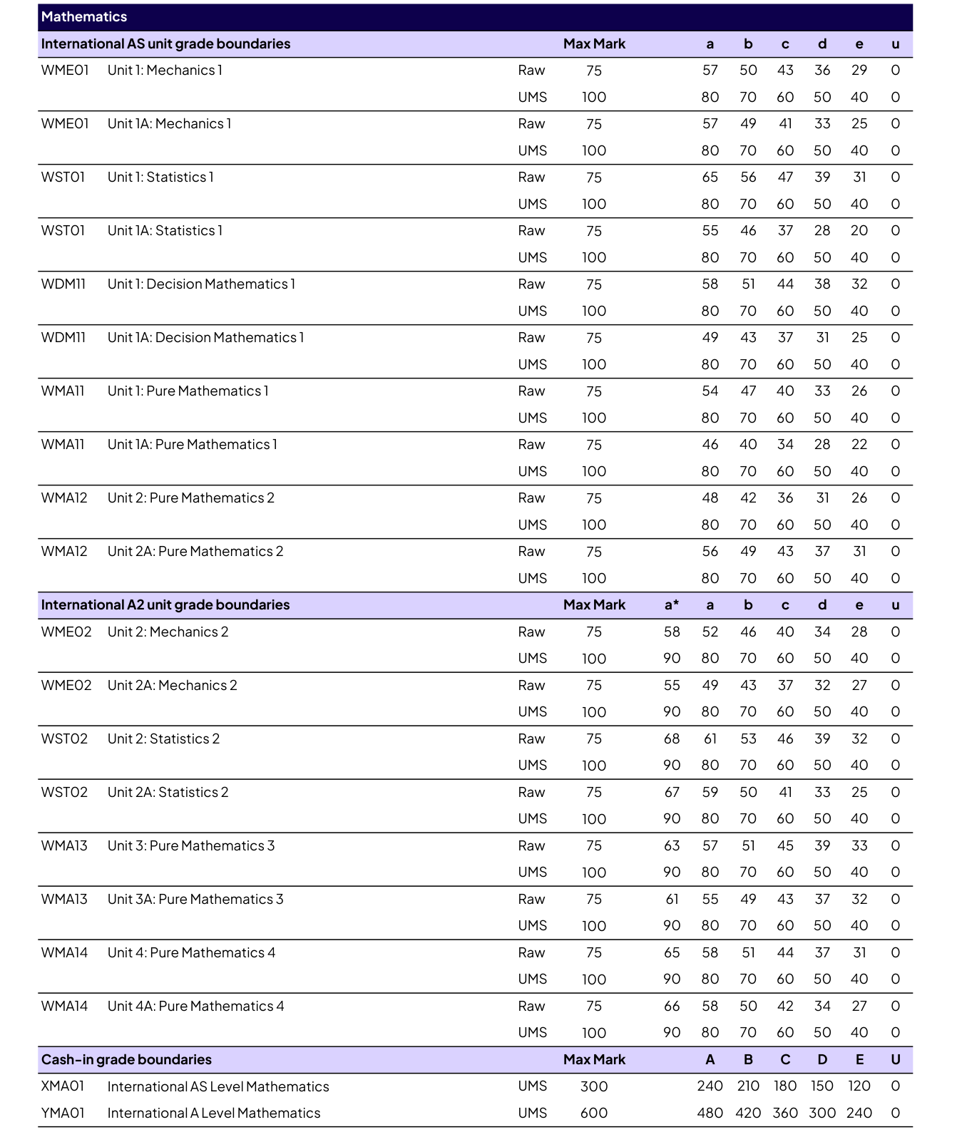
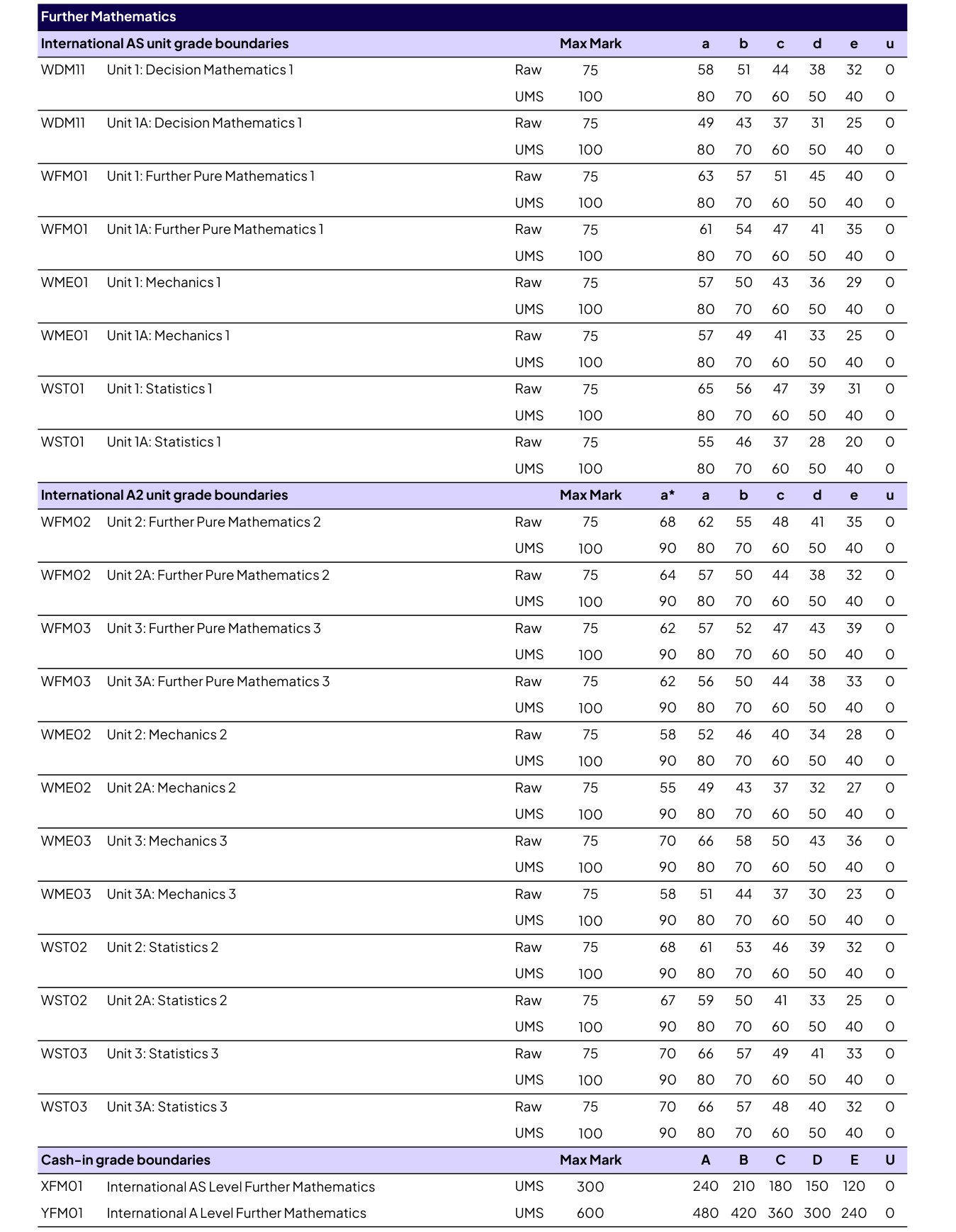
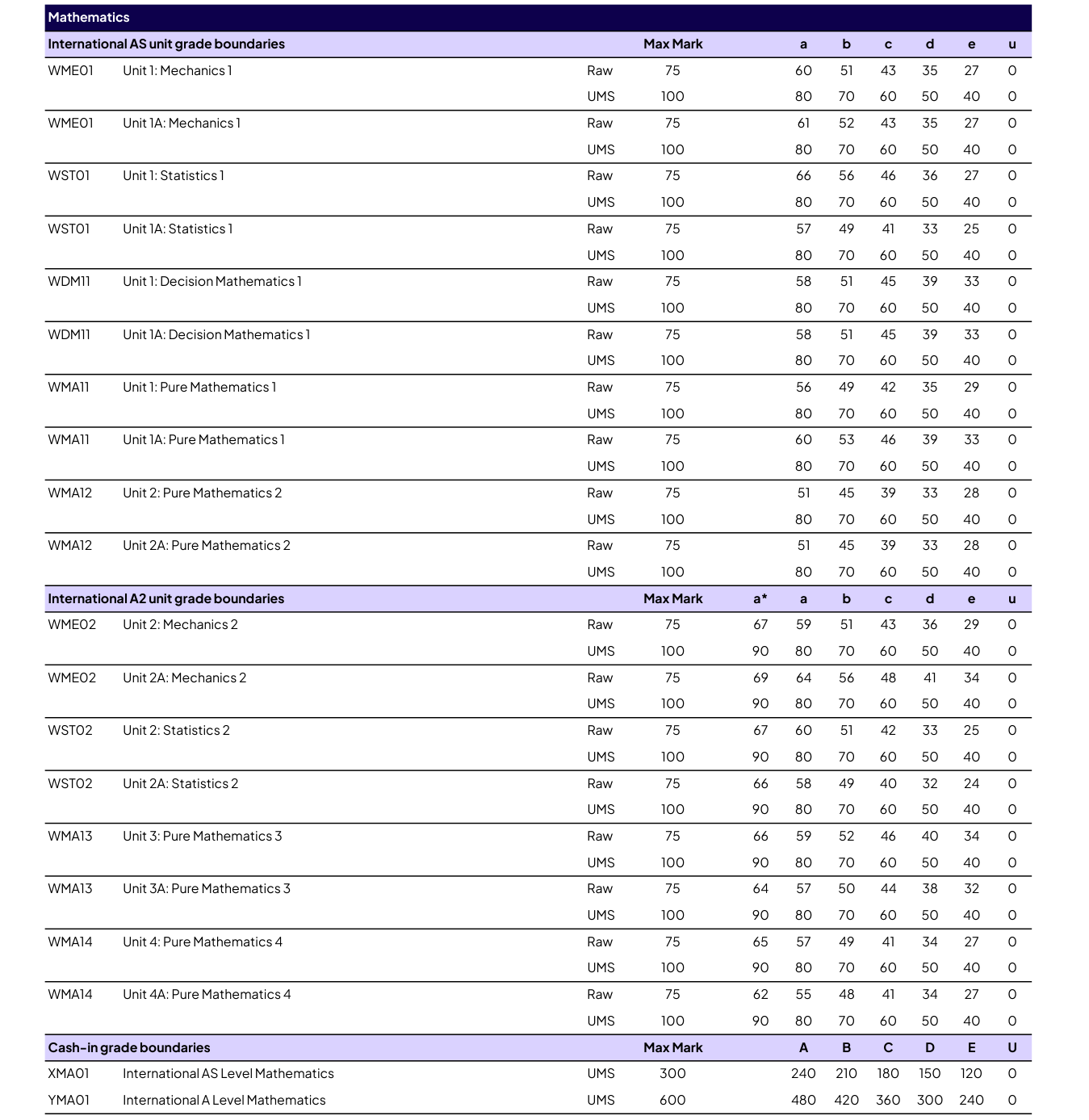
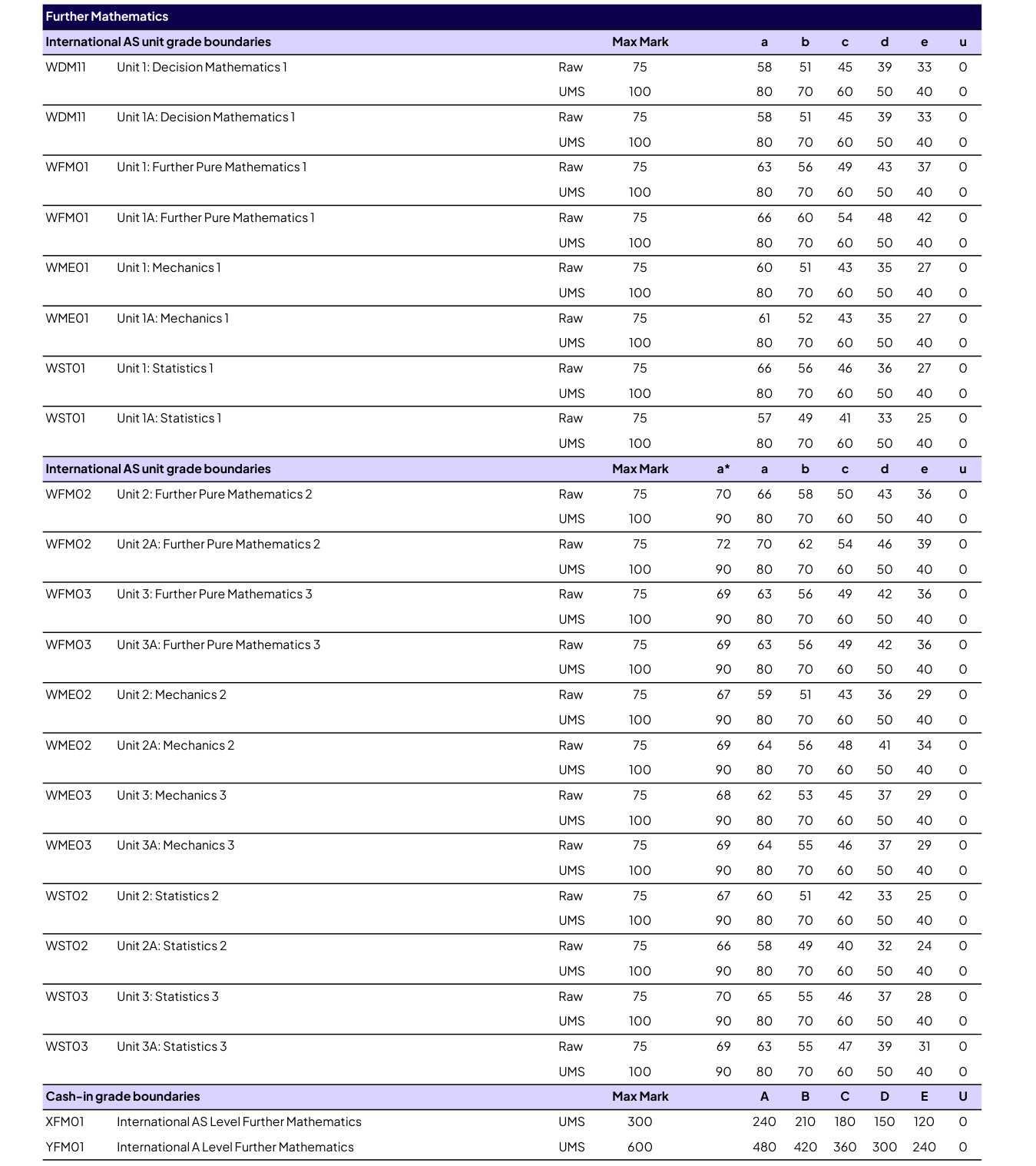
每次考季后 Pearson 按当次试卷难度公布各单元的 Raw(原始分)分界;UMS 分界固定不变(AS 单元 a–e 对应 80/70/60/50/40,A2 单元另设 a* = 90)。表中同一单元的两行(如 Unit 1 与 Unit 1A)为同一份试卷的不同版本,Raw 分界不同、UMS 分界相同,具体以考生所考版本为准。
📍 2026年6月考季
📍 2026年1月考季
📍 2025年10月考季
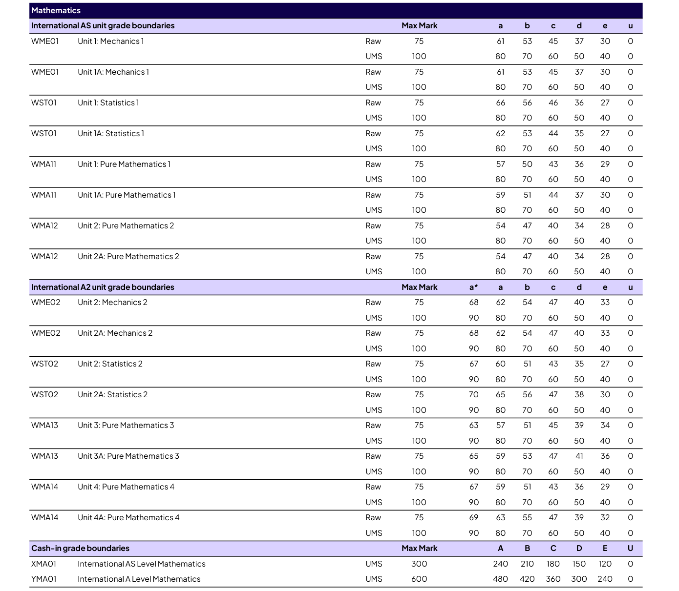
截图来源:qualifications.pearson.com 官方「Grade boundaries — International A Level」文件(2026 年 6 月 / 2026 年 1 月 / 2025 年 10 月考季)。2025 年 10 月考季官方文件未含进阶数学段落(该考季未开放相应单元)。
📝 S3 分类真题 Categorised Past Papers
Edexcel IAL WST03 (S3) 2019–2026 共 15 卷 / 106 题(含 01A 区域变体), 按官方规格 6 个章节、20 个知识点双语分类。点开任一知识点即可看到对应年份的真题; 每题附「题目 Question」与「详解 Mark Scheme」两个链接,均为所在完整试卷页原版(PDF 整页,不裁剪)。
同一知识点可能出现在多个章节之下(各章只列属于该章的题)。
1 · 随机变量的组合 Combinations of random variables (15 题)
线性组合的期望与方差 E and Var of linear combinations (1 题)
| 试卷 Session | 题号 | 分值 | 链接 Links |
|---|---|---|---|
| 2023 Jun | Q7 | 10 | 题目 Question · 详解 Mark Scheme |
独立正态变量的组合 Combining independent normal variables (15 题)
| 试卷 Session | 题号 | 分值 | 链接 Links |
|---|---|---|---|
| 2019 Jun | Q8 | 13 | 题目 Question · 详解 Mark Scheme |
| 2020 Oct | Q7 | 16 | 题目 Question · 详解 Mark Scheme |
| 2021 Jun | Q6 | 17 | 题目 Question · 详解 Mark Scheme |
| 2022 Jan | Q5 | 17 | 题目 Question · 详解 Mark Scheme |
| 2022 Jun | Q6 | 10 | 题目 Question · 详解 Mark Scheme |
| 2023 Jan | Q7 | 8 | 题目 Question · 详解 Mark Scheme |
| 2023 Jun | Q7 | 10 | 题目 Question · 详解 Mark Scheme |
| 2024 Jan | Q7 | 14 | 题目 Question · 详解 Mark Scheme |
| 2024 Jun | Q6 | 16 | 题目 Question · 详解 Mark Scheme |
| 2025 Jan | Q7 | 15 | 题目 Question · 详解 Mark Scheme |
| 2025 Jun | Q8 | 15 | 题目 Question · 详解 Mark Scheme |
| 2026 Jan | Q8 | 13 | 题目 Question · 详解 Mark Scheme |
| 2026 Jan 01A | Q7 | 15 | 题目 Question · 详解 Mark Scheme |
| 2026 Jun | Q7 | 12 | 题目 Question · 详解 Mark Scheme |
| 2026 Jun 01A | Q6 | 16 | 题目 Question · 详解 Mark Scheme |
2 · 抽样 Sampling (4 题)
抽样方法与比较 Sampling methods and comparisons (4 题)
| 试卷 Session | 题号 | 分值 | 链接 Links |
|---|---|---|---|
| 2019 Jun | Q1 | 4 | 题目 Question · 详解 Mark Scheme |
| 2024 Jan | Q2 | 7 | 题目 Question · 详解 Mark Scheme |
| 2024 Jun | Q1 | 4 | 题目 Question · 详解 Mark Scheme |
| 2025 Jun | Q1 | 3 | 题目 Question · 详解 Mark Scheme |
3 · 有偏与无偏估计量 Biased & unbiased estimators (8 题)
µ 与 σ² 的无偏估计 Unbiased estimators of µ and σ² (2 题)
| 试卷 Session | 题号 | 分值 | 链接 Links |
|---|---|---|---|
| 2022 Jun | Q5 | 9 | 题目 Question · 详解 Mark Scheme |
| 2026 Jan | Q7 | 8 | 题目 Question · 详解 Mark Scheme |
有偏无偏的判定与比较 Determining and comparing bias (7 题)
| 试卷 Session | 题号 | 分值 | 链接 Links |
|---|---|---|---|
| 2020 Oct | Q1 | 4 | 题目 Question · 详解 Mark Scheme |
| 2022 Jun | Q5 | 9 | 题目 Question · 详解 Mark Scheme |
| 2023 Jun | Q3 | 9 | 题目 Question · 详解 Mark Scheme |
| 2025 Jan | Q6 | 9 | 题目 Question · 详解 Mark Scheme |
| 2025 Jun | Q6 | 8 | 题目 Question · 详解 Mark Scheme |
| 2026 Jan 01A | Q2 | 7 | 题目 Question · 详解 Mark Scheme |
| 2026 Jun 01A | Q3 | 11 | 题目 Question · 详解 Mark Scheme |
4 · 置信区间与显著性检验 Confidence intervals and significance tests (37 题)
抽样分布与标准误 Sampling distribution of the mean and standard error (5 题)
| 试卷 Session | 题号 | 分值 | 链接 Links |
|---|---|---|---|
| 2023 Jan | Q6 | 10 | 题目 Question · 详解 Mark Scheme |
| 2023 Jun | Q5 | 13 | 题目 Question · 详解 Mark Scheme |
| 2024 Jan | Q6 | 15 | 题目 Question · 详解 Mark Scheme |
| 2025 Jun | Q7 | 11 | 题目 Question · 详解 Mark Scheme |
| 2026 Jan | Q6 | 8 | 题目 Question · 详解 Mark Scheme |
中心极限定理 Central limit theorem (9 题)
| 试卷 Session | 题号 | 分值 | 链接 Links |
|---|---|---|---|
| 2019 Jun | Q4 | 6 | 题目 Question · 详解 Mark Scheme |
| 2019 Jun | Q5 | 8 | 题目 Question · 详解 Mark Scheme |
| 2020 Oct | Q6 | 8 | 题目 Question · 详解 Mark Scheme |
| 2021 Jun | Q4 | 16 | 题目 Question · 详解 Mark Scheme |
| 2022 Jan | Q2 | 8 | 题目 Question · 详解 Mark Scheme |
| 2022 Jun | Q4 | 10 | 题目 Question · 详解 Mark Scheme |
| 2024 Jun | Q7 | 8 | 题目 Question · 详解 Mark Scheme |
| 2026 Jun | Q6 | 9 | 题目 Question · 详解 Mark Scheme |
| 2026 Jun 01A | Q7 | 7 | 题目 Question · 详解 Mark Scheme |
置信区间 Confidence intervals (16 题)
| 试卷 Session | 题号 | 分值 | 链接 Links |
|---|---|---|---|
| 2019 Jun | Q4 | 6 | 题目 Question · 详解 Mark Scheme |
| 2020 Oct | Q6 | 8 | 题目 Question · 详解 Mark Scheme |
| 2021 Jun | Q3 | 8 | 题目 Question · 详解 Mark Scheme |
| 2022 Jan | Q1 | 10 | 题目 Question · 详解 Mark Scheme |
| 2022 Jun | Q3 | 14 | 题目 Question · 详解 Mark Scheme |
| 2023 Jan | Q6 | 10 | 题目 Question · 详解 Mark Scheme |
| 2023 Jun | Q5 | 13 | 题目 Question · 详解 Mark Scheme |
| 2024 Jan | Q6 | 15 | 题目 Question · 详解 Mark Scheme |
| 2024 Jun | Q3 | 12 | 题目 Question · 详解 Mark Scheme |
| 2024 Jun | Q7 | 8 | 题目 Question · 详解 Mark Scheme |
| 2025 Jan | Q4 | 12 | 题目 Question · 详解 Mark Scheme |
| 2026 Jan | Q3 | 8 | 题目 Question · 详解 Mark Scheme |
| 2026 Jan 01A | Q4 | 7 | 题目 Question · 详解 Mark Scheme |
| 2026 Jun | Q5 | 12 | 题目 Question · 详解 Mark Scheme |
| 2026 Jun 01A | Q4 | 10 | 题目 Question · 详解 Mark Scheme |
| 2026 Jun 01A | Q7 | 7 | 题目 Question · 详解 Mark Scheme |
置信区间宽度与样本量 Confidence interval width and sample size (3 题)
| 试卷 Session | 题号 | 分值 | 链接 Links |
|---|---|---|---|
| 2022 Jun | Q3 | 14 | 题目 Question · 详解 Mark Scheme |
| 2025 Jan | Q4 | 12 | 题目 Question · 详解 Mark Scheme |
| 2026 Jun | Q5 | 12 | 题目 Question · 详解 Mark Scheme |
均值检验(方差已知) Hypothesis test for a mean (variance known) (5 题)
| 试卷 Session | 题号 | 分值 | 链接 Links |
|---|---|---|---|
| 2019 Jun | Q6 | 14 | 题目 Question · 详解 Mark Scheme |
| 2021 Jun | Q4 | 16 | 题目 Question · 详解 Mark Scheme |
| 2023 Jan | Q1 | 12 | 题目 Question · 详解 Mark Scheme |
| 2023 Jan | Q5 | 10 | 题目 Question · 详解 Mark Scheme |
| 2024 Jun | Q3 | 12 | 题目 Question · 详解 Mark Scheme |
均值检验(方差未知/大样本) Hypothesis test for a mean (variance unknown, large sample) (13 题)
| 试卷 Session | 题号 | 分值 | 链接 Links |
|---|---|---|---|
| 2019 Jun | Q6 | 14 | 题目 Question · 详解 Mark Scheme |
| 2020 Oct | Q5 | 12 | 题目 Question · 详解 Mark Scheme |
| 2022 Jan | Q2 | 8 | 题目 Question · 详解 Mark Scheme |
| 2022 Jun | Q2 | 11 | 题目 Question · 详解 Mark Scheme |
| 2023 Jun | Q6 | 13 | 题目 Question · 详解 Mark Scheme |
| 2024 Jan | Q5 | 9 | 题目 Question · 详解 Mark Scheme |
| 2024 Jun | Q5 | 14 | 题目 Question · 详解 Mark Scheme |
| 2025 Jan | Q3 | 12 | 题目 Question · 详解 Mark Scheme |
| 2025 Jun | Q4 | 11 | 题目 Question · 详解 Mark Scheme |
| 2026 Jan | Q5 | 12 | 题目 Question · 详解 Mark Scheme |
| 2026 Jan 01A | Q6 | 17 | 题目 Question · 详解 Mark Scheme |
| 2026 Jun | Q3 | 11 | 题目 Question · 详解 Mark Scheme |
| 2026 Jun 01A | Q2 | 11 | 题目 Question · 详解 Mark Scheme |
5 · 拟合优度与 χ² 检验 Goodness of fit, χ² test (27 题)
自由度与合并项 Degrees of freedom and pooling classes (8 题)
| 试卷 Session | 题号 | 分值 | 链接 Links |
|---|---|---|---|
| 2019 Jun | Q7 | 9 | 题目 Question · 详解 Mark Scheme |
| 2021 Jun | Q5 | 16 | 题目 Question · 详解 Mark Scheme |
| 2022 Jan | Q6 | 14 | 题目 Question · 详解 Mark Scheme |
| 2023 Jan | Q4 | 14 | 题目 Question · 详解 Mark Scheme |
| 2023 Jun | Q4 | 11 | 题目 Question · 详解 Mark Scheme |
| 2024 Jan | Q4 | 10 | 题目 Question · 详解 Mark Scheme |
| 2024 Jun | Q4 | 11 | 题目 Question · 详解 Mark Scheme |
| 2025 Jan | Q2 | 7 | 题目 Question · 详解 Mark Scheme |
离散均匀分布拟合 Goodness of fit: discrete uniform (2 题)
| 试卷 Session | 题号 | 分值 | 链接 Links |
|---|---|---|---|
| 2020 Oct | Q4 | 15 | 题目 Question · 详解 Mark Scheme |
| 2022 Jun | Q7 | 11 | 题目 Question · 详解 Mark Scheme |
二项分布拟合 Goodness of fit: binomial (5 题)
| 试卷 Session | 题号 | 分值 | 链接 Links |
|---|---|---|---|
| 2021 Jun | Q5 | 16 | 题目 Question · 详解 Mark Scheme |
| 2023 Jan | Q4 | 14 | 题目 Question · 详解 Mark Scheme |
| 2025 Jun | Q5 | 11 | 题目 Question · 详解 Mark Scheme |
| 2026 Jan | Q4 | 12 | 题目 Question · 详解 Mark Scheme |
| 2026 Jun | Q4 | 13 | 题目 Question · 详解 Mark Scheme |
泊松分布拟合 Goodness of fit: Poisson (4 题)
| 试卷 Session | 题号 | 分值 | 链接 Links |
|---|---|---|---|
| 2019 Jun | Q7 | 9 | 题目 Question · 详解 Mark Scheme |
| 2024 Jan | Q4 | 10 | 题目 Question · 详解 Mark Scheme |
| 2025 Jan | Q2 | 7 | 题目 Question · 详解 Mark Scheme |
| 2026 Jan 01A | Q5 | 9 | 题目 Question · 详解 Mark Scheme |
正态分布拟合 Goodness of fit: normal (1 题)
| 试卷 Session | 题号 | 分值 | 链接 Links |
|---|---|---|---|
| 2022 Jan | Q6 | 14 | 题目 Question · 详解 Mark Scheme |
列联表独立性检验 Contingency tables: independence (χ²) tests (13 题)
| 试卷 Session | 题号 | 分值 | 链接 Links |
|---|---|---|---|
| 2019 Jun | Q2 | 10 | 题目 Question · 详解 Mark Scheme |
| 2020 Oct | Q2 | 9 | 题目 Question · 详解 Mark Scheme |
| 2021 Jun | Q2 | 9 | 题目 Question · 详解 Mark Scheme |
| 2022 Jan | Q4 | 14 | 题目 Question · 详解 Mark Scheme |
| 2023 Jan | Q3 | 9 | 题目 Question · 详解 Mark Scheme |
| 2023 Jun | Q2 | 10 | 题目 Question · 详解 Mark Scheme |
| 2024 Jan | Q1 | 8 | 题目 Question · 详解 Mark Scheme |
| 2025 Jan | Q5 | 12 | 题目 Question · 详解 Mark Scheme |
| 2025 Jun | Q3 | 9 | 题目 Question · 详解 Mark Scheme |
| 2026 Jan | Q1 | 8 | 题目 Question · 详解 Mark Scheme |
| 2026 Jan 01A | Q3 | 12 | 题目 Question · 详解 Mark Scheme |
| 2026 Jun | Q2 | 9 | 题目 Question · 详解 Mark Scheme |
| 2026 Jun 01A | Q5 | 11 | 题目 Question · 详解 Mark Scheme |
6 · 回归与相关 Regression and correlation (15 题)
斯皮尔曼等级相关 Spearman's rank correlation (15 题)
| 试卷 Session | 题号 | 分值 | 链接 Links |
|---|---|---|---|
| 2019 Jun | Q3 | 11 | 题目 Question · 详解 Mark Scheme |
| 2020 Oct | Q3 | 11 | 题目 Question · 详解 Mark Scheme |
| 2021 Jun | Q1 | 9 | 题目 Question · 详解 Mark Scheme |
| 2022 Jan | Q3 | 12 | 题目 Question · 详解 Mark Scheme |
| 2022 Jun | Q1 | 10 | 题目 Question · 详解 Mark Scheme |
| 2023 Jan | Q2 | 12 | 题目 Question · 详解 Mark Scheme |
| 2023 Jun | Q1 | 9 | 题目 Question · 详解 Mark Scheme |
| 2024 Jan | Q3 | 12 | 题目 Question · 详解 Mark Scheme |
| 2024 Jun | Q2 | 10 | 题目 Question · 详解 Mark Scheme |
| 2025 Jan | Q1 | 8 | 题目 Question · 详解 Mark Scheme |
| 2025 Jun | Q2 | 7 | 题目 Question · 详解 Mark Scheme |
| 2026 Jan | Q2 | 6 | 题目 Question · 详解 Mark Scheme |
| 2026 Jan 01A | Q1 | 8 | 题目 Question · 详解 Mark Scheme |
| 2026 Jun | Q1 | 9 | 题目 Question · 详解 Mark Scheme |
| 2026 Jun 01A | Q1 | 9 | 题目 Question · 详解 Mark Scheme |
零相关检验(PMCC) Testing for zero correlation (PMCC) (4 题)
| 试卷 Session | 题号 | 分值 | 链接 Links |
|---|---|---|---|
| 2022 Jan | Q3 | 12 | 题目 Question · 详解 Mark Scheme |
| 2023 Jan | Q2 | 12 | 题目 Question · 详解 Mark Scheme |
| 2023 Jun | Q1 | 9 | 题目 Question · 详解 Mark Scheme |
| 2024 Jan | Q3 | 12 | 题目 Question · 详解 Mark Scheme |
并列秩的处理 Tied ranks (2 题)
| 试卷 Session | 题号 | 分值 | 链接 Links |
|---|---|---|---|
| 2020 Oct | Q3 | 11 | 题目 Question · 详解 Mark Scheme |
| 2022 Jun | Q1 | 10 | 题目 Question · 详解 Mark Scheme |
真题版权归 Pearson Edexcel 所有,此处仅作教学练习用途。
同一考季只保留一条链接:QP(试卷)/ MS(评分表)优先用 Pearson 官方直链,官方未公开该考季时才回退到第三方镜像 PMT(physicsandmathstutor.com,链接带 <em>PMT</em> 小标签);MA(Model Answers 详解)仅 PMT 有,ER(Examiner Report 考官报告)仅官方有。
⚠️ October 2025 / January 2026 / June 2026 三个考季:官方材料已上传但锁在教师账号后(访问跳登录页),第三方也尚未收录——本站不提供这三个考季的链接,需要请登录 Pearson 官方 course materials 页或经所在 centre 获取。
同一次考试可能有多个版本(如 Unit 1 与 Unit 1A),另有少量“(Unused)”备用卷,以表中实际列为准。
📄 Statistics 3(WST03)· 历年真题与评分材料
| 考季 | 试卷 QP | 评分表 MS | 详解 MA | 考官报告 ER |
|---|---|---|---|---|
| October 2020 | QP | MS PMT | – | – |
| January 2021 | QP PMT | MS | – | – |
| June 2021 | QP | MS | – | – |
| October 2021 | QP | MS PMT | – | ER |
| January 2022 | QP PMT | MS PMT | – | – |
| June 2022 | QP | MS | – | ER |
| January 2023 | QP | MS | – | ER |
| June 2023 | QP | MS | – | ER |
| January 2024 | QP | MS | – | ER |
| June 2024 | QP | MS | – | ER |
| January 2025 | QP | MS | – | ER |
| June 2025 | QP | MS | – | ER |
本单元索引页:PMT https://www.physicsandmathstutor.com/a-level-maths-papers/edexcel-maths-ial-papers/; Pearson 官方 Mathematics (2018) course materials(需教师账号的考季也在这里登录获取)。
QP = Question paper 试卷 · MS = Mark scheme 评分表 · MA = Model answers 详解 · ER = Examiner report 考官报告。 未带小标签的为 **Pearson 官方**直链;带 PMT 小标签的为第三方镜像(physicsandmathstutor.com)。 同一考季同一文档只保留一条链接,官方优先。全部链接 2026-10-15 逐条实测可下载。