该板块暂无内容。
内容稍后补充。
1统计建模Statistical modelling
统计建模Statistical modelling
Example:When a die is rolled, we say that the probability of each number is 16. This is a statistical model, but the assumption that each face is equally likely might not be true. Suppose the die is weighted to increase the chance of a six. We might then find, after experimenting, that the probability of a six is 14 and the probability of a one is 112, with the probability of other faces remaining at 16, all adding up to 1. In this case we have refined, or improved, the model to give a truer picture.
Example:The heights of a large group of adults are measured. The mean is 172⋅3 cm and the standard deviation is 12⋅4 cm.
It could be thought that the general shape of the histogram can be modelled by the curve
This might not give a true picture, in which case we would have to change the equation, or refine the model.
定义Definition
一个统计模型是对真实世界情境的简化,通常用方程来描述真实世界的情境。它可以用来对真实世界的问题作出预测。通过分析和修正模型,可以获得更深入的理解。
优点Advantages
- 模型快速且易于建立
- 模型有助于我们理解真实世界的问题
- 模型有助于我们作出预测
- 模型有助于我们控制某种情境 – 例如铁路时刻表、空中交通管制等。
缺点Disadvantages
- 模型简化了情境,只描述了真实世界问题的一部分。
- 模型可能只在某些情境下成立,或只适用于特定的取值范围。
2样本数据的表示Representation of sample data
变量Variables
定性变量Qualitative variables
非数值 - 例如 红色、蓝色,或 长、短 等。
定量变量Quantitative variables
数值 - 例如 长度、年龄、时间、口袋中硬币的枚数 等。
连续变量Continuous variables
可以取给定范围内的任意值 - 例如 身高、时间、年龄 等。
离散变量Discrete variables
只能取某些特定的值 - 例如 鞋码、以 £ 和 p 计的价格、硬币的枚数。
频数分布Frequency distributions
频数分布表Frequency distribution
一个分布最好理解成一张表。因此,一个频数分布可以看作一张频数表,即一列离散取值及其对应的频数。
Example:The number of M&Ms is counted in several bags, and recorded in the frequency distribution/table below:
| number of M&Ms | 37 | 38 | 39 | 40 | 41 | 42 | 43 |
|---|---|---|---|---|---|---|---|
| frequency | 3 | 8 | 11 | 19 | 13 | 7 | 2 |
累积频数Cumulative frequency
沿着列表向下(或向右)把频数逐项累加。
| M&M 豆的个数 | 37 | 38 | 39 | 40 | 41 | 42 | 43 |
|---|---|---|---|---|---|---|---|
| 频数 | 3 | 8 | 11 | 19 | 13 | 7 | 2 |
| 累积频数 | 3 | 11 | 22 | 41 | 54 | 61 | 63 |
茎叶图与背靠背茎叶图Stem and leaf & back-to-back stem and leaf diagrams
把各位数字作为叶依次排在枝上,使它看起来像一张条形图。
每根枝上的叶必须按数值顺序排列,从茎开始。
加上一个图例;例如 5|2 表示 52,或 4|3 表示 4⋅3 等。
由背靠背茎叶图比较两个分布Comparing two distributions from a back to back stem and leaf diagram.
比较:
- A 中的数值平均而言比 B 中的小。
- A 中的数值比 B 中的更分散。
通过观察这张图,你总能作出至少两条比较:通常一条关于中位数,另一条关于离散程度,往往是四分位距。
分组频数分布Grouped frequency distributions
组界与组距Class boundaries and widths
在确定组界时,一个组与下一个组之间绝不能留下空隙,无论处理的是连续分布还是离散分布。
对于离散分布,用组界可以避免组与组之间留下空隙,如下所示: X = 0, 1, 2, 3, 4, 5, 6, 7, … 离散。
| 组区间(原样) | 组中包含的值 | 无空隙的组界 |
|---|---|---|
| 0 – 4 | 0, 1, 2, 3, 4 | 0 – 4⋅5 |
| 5 – 9 | 5, 6, 7, 8, 9 | 4⋅5– 9⋅5 |
| 10 – 12 | 10, 11, 12 | 9⋅5 – 12⋅5 |
| 等 |
对于连续分布,组界可以取在任何位置。
分组数据的累积频数曲线Cumulative frequency curves for grouped data
Example:0 ≤ x < 5, 5 ≤ x < 9, 9 ≤ x < 16, etc.
Note that each interval starts at the point where the previous interval ended, but 5, for example, goes in the second interval 5 ≤ x < 9.
对于离散频数分布表。
| 组区间 | 组界 | 频数 | 组 | 累积频数 |
|---|---|---|---|---|
| 0 - 4 | 0 to 4⋅5 | 27 | ≤ 4⋅5 | 27 |
| 5 – 9 | 4⋅5 to 9⋅5 | 36 | ≤ 9⋅5 | 63 |
| 10 – 19 | 9⋅5 to 19⋅5 | 54 | ≤ 19⋅5 | 117 |
| 20 – 29 | 19⋅5 to 29⋅5 | 49 | ≤ 29⋅5 | 166 |
| 30 – 59 | 29⋅5 to 59⋅5 | 24 | ≤ 59⋅5 | 190 |
| 60 –99 | 59⋅5 to 99⋅5 | 10 | ≤ 99⋅5 | 200 |
在区间的端点处描点,例如 (4⋅5, 27)、(9⋅5, 63)、(19⋅5, 117) 等,再用一条平滑曲线把这些点连起来。
直方图Histograms
直方图处理的是连续数据。条形之间不留空隙。
因此,当我们有下列组区间时,它们必须理解为:
要画直方图,先列出一张表,写出组区间、组界、组距和频数,然后每一根条形的高度按下式计算:
(这个高度称为频数密度):
| 组区间 | 组界 | 组距 | 频数 | 频数密度 |
|---|---|---|---|---|
| 0 - 4 | 0 to 4⋅5 | 4⋅5 | 27 | 6 |
| 5 – 9 | 4⋅5 to 9⋅5 | 5 | 36 | 7⋅2 |
| 10 – 19 | 9⋅5 to 19⋅5 | 10 | 54 | 5⋅4 |
| 20 – 29 | 19⋅5 to 29⋅5 | 10 | 49 | 4⋅9 |
| 30 – 44 | 29⋅5 to 44⋅5 | 15 | 24 | 1⋅6 |
| 45 –59 | 44⋅5 to 59⋅5 | 15 | 12 | 0⋅8 |
在上面的图和表中我们看到,最高的那根条形不一定是频数最大的,而是频数密度最大的。条形最高的是 4⋅5 – 9⋅5 这一组,而频数最大的是 9⋅5 – 19⋅5 这一组(它实际上是第三高的条形)。
在这个例子中我们取了 频数密度 × 组距 = 面积。情况并非总是如此,但 频数密度 × 组距 总是与面积成正比。
Example:100 people were asked how many DVDs they owned. The results are shown below.
| Number of DVDs | frequency |
|---|---|
| 12 to 14 | 15 |
| 15 to 16 | |
| 17 | |
| 18 to 21 | |
| 22 to 30 |
(a) What are the class boundaries for the interval 12 to 14?
(b) What is the area of the bar for the class 12 to 14? Compare this with the frequency for this class.
(c) Fill in the blanks in the frequency table. Check that your frequencies add up to 100.
(d) Find the number of people who own between 15 and 24 DVDs, inclusive.
Solution:
(a) Class boundaries for the interval 12 to 14 are 11⋅5 to 14⋅5
(b) Class width of bar for 12 to 14 is 14⋅5 – 11⋅5 = 3, height of bar = 2⋅5, ⇒ area = 3 × 2⋅5 = 7⋅5 which is half the frequency, 15.
Thus the frequency is always twice the area.
(c) 15 to 16 is 14⋅5 to 16⋅5 width 2, height 4⋅5 ⇒ area 9 ⇒ frequency = 2× 9 = 18
17 is 16⋅5 to 17⋅5 width 1, height 8⋅5 ⇒ area 8⋅5 ⇒ frequency = 2× 8⋅5 = 17
18 to 21 is 17⋅5 to 21⋅5 width 4, height 4 ⇒ area 16 ⇒ frequency = 2 × 16 = 32
22 to 30 is 21⋅5 to 30⋅5 width 9, height 1 ⇒ area 9 ⇒ frequency = 2× 9 = 18
Check 15 + 18 + 17 + 32 + 18 = 100, which is correct
(d) 15 to 24 is 14⋅5 to 24⋅5
14⋅5 to 16⋅5 and 16⋅5 to 17⋅5 and 17⋅5 to 21⋅5 gives f = 18 + 17 + 32
21⋅5 to 24⋅5 has width 3 and height 1 so area = 3 ⇒ f = 2 × 3 = 6
⇒ number between 15 and 24 inclusive is 18 + 17 + 32 + 6 = 73.
以厘米为单位的宽度与高度Width and height in centimetres
当宽度和高度以厘米为单位、面积以平方厘米为单位时:
组距与以厘米为单位的宽度成正比,
频数密度与以厘米为单位的高度成正比,
而频数与条形以平方厘米为单位的面积成正比。
频数可能等于条形的面积,可能是面积的两倍,也可能是面积的三分之一,等等。
Example:A histogram is to be drawn from the following data:
| x | f |
|---|---|
| 2 − 4 | 15 |
| 5 − 6 | 9 |
| 7 − 12 | 18 |
| 13 − 16 | 10 |
The width of the 2 − 4 interval is 6 cm, and its height is 8 cm.
Find the widths and heights, in cm, for the 5 − 6, the 7 − 12, and the 13 − 16 bars.
Solution:
(a) The 2 − 4 interval has width 6 cm, height 8 cm ⇒ area = 6 × 8 = 48 cm 2.
The 2 − 4 interval is 1⋅5 to 4⋅5, so has width 3 ∝ 6 cm and frequency 15 ∝ 48 cm2.
(b) The 5 − 6 interval is 4⋅5 − 6⋅5, so has width 2, which is 23 of the width of the 2 to 4 interval, so its width (in cm) is 23× 6 = 4 cm.
The 5 − 6 bar has a frequency of 6, which is 615 of the frequency of the 2 − 4 bar, so the area of the 5 − 6 bar is 615× 48 = 19⋅2 cm2,
⇒ height is area ÷ width = 19⋅2 cm2 ÷ 4 cm = 4⋅8 cm.
(c) We can now fill in the table below, working from left to right.
| x | boundaries | width | frequency | width, cm | area, cm2 | height, cm |
|---|---|---|---|---|---|---|
| 2 − 4 | 1⋅5 – 4⋅5 | 3 | 15 | 6 cm | 6 cm × 8 cm = 48 cm2 | 8 cm |
| 5 − 6 | 4⋅5 – 6⋅5 | 2 | 9 | 23× 6 = 4 cm | 915× 48 = 28⋅8 cm2 | 28⋅8 ÷ 4 = 7⋅2 cm |
| 7 − 12 | 6⋅5 – 12⋅5 | 6 | 18 | 63× 6 = 12 cm | 1815× 48 = 57⋅6 cm2 | 57⋅6 ÷ 12 = 4⋅8 cm |
| 13 − 16 | 12⋅5 – 16⋅5 | 4 | 10 | 43× 6 = 8 cm | 1015× 48 = 32 cm2 | 32 ÷ 8 = 4 cm |
Example:A grouped frequency table for the weights of adults has the following entries:
| weight kg | … | … | 50 – 60 | 60 – 70 | 70 – 85 | … |
|---|---|---|---|---|---|---|
| frequency | … | … | 60 | 35 | 20 | … |
In a histogram, the bar for the class 50 – 60 kg is 2 cm wide and 9 cm high.
Find the width and height of the bar for the 70 – 85 kg class.
Solution:50 – 60 is usually taken to mean 50 ≤ weight < 60
The width of the 50 – 60 class is 10 kg ≡ 2 cm
The area of the 50 – 60 bar is 2 cm × 9 cm = 18 cm2 ⇔ frequency is 60
Answer the width of 70 – 85 kg bar is 3 cm, and the height is 2 cm.
3众数与平均数(及中位数)Mode, mean (and median)
众数Mode
众数是出现次数最多的取值或组区间。
平均数Mean
对于取值 x1, x2, … , xn 与频数 f1, f2, … , fn,平均数为
Example:Find the mean for the following table showing the number of children per family.
Solution:
| Number of children | Frequency | |
|---|---|---|
| x | f | xf |
| 0 | 5 | 0 |
| 1 | 8 | 8 |
| 2 | 12 | 24 |
| 3 | 18 | 54 |
| 4 | 9 | 36 |
| 5 | 4 | 20 |
| 56 | 142 |
Σ xifi = 142, and N = Σ fi = 56
⇒ x = 14256 = 2⋅54 to 3 S.F.
注意,平均数 m 常写作 m = 1Nn∑1xi,而 fi 省略不写。
在分组频数表中必须使用组中值。
Example:The table shows the numbers of children in prep school classes in a town.
Solution:
| Number of children | Mid-interval value | Frequency | |
|---|---|---|---|
| x | f | xf | |
| 1 - 10 | 5⋅5 | 5 | 27⋅5 |
| 11 - 15 | 13 | 8 | 104 |
| 16 – 20 | 18 | 12 | 216 |
| 21 - 30 | 25⋅5 | 18 | 459 |
| 31 - 40 | 35⋅5 | 11 | 390⋅5 |
| 54 | 1197 |
Σ xi fi = 1197, and N = Σ fi = 54
⇒ x = 119754 = 22⋅2 to 3 S.F.
编码Coding
一组人的体重以千克为单位给出,记为 x1, x2, … xn。现在把这些体重改为以克为单位,记为 t1, t2, … tn。
在这里 ti = 1000 × xi – 这就是编码的一个例子。
编码的另一个例子可以是 ti = xi−205 .
编码与平均数的计算Coding and calculating the mean
采用编码 ti = xi−205 时,我们从每个 x 值中减去 20,再把结果除以 5。
我们先求出 ti 的平均数,再逆向运算求出 xi 的平均数。
⇒ 先求 ti 的平均数,再乘以 5 并加上 20,得到 x = 5t + 20。
因为 t = 1Nn∑i=1tifi,且 N = n∑i=1fi
Example:Use the coding ti = xi−16510 to find the mean weight for the following distribution.
| Weight, kg | Mid-interval | Coded value | Frequency | |
|---|---|---|---|---|
| xi | ti = xi−16510 | fi | tifi | |
| 140 - 150 | 145 | –2 | 9 | –18 |
| 150 - 160 | 155 | –1 | 21 | –21 |
| 160 - 170 | 165 | 0 | 37 | 0 |
| 170 - 180 | 175 | 1 | 28 | 28 |
| 180 - 190 | 185 | 2 | 11 | 22 |
| 106 | 11 |
⇒ t = 11106
and ti = xi−16510 ⇒ x = 10 t + 165 = 10 × 11106 + 165 = 166⋅0377358
⇒ mean weight is 166⋅04 kg to 2 D.P.
在这里,编码为那些喜欢不用计算器的人简化了算术运算!
中位数Median
中位数是有序数列中最中间的那个数。中位数的求法将在下一节说明。
何时使用众数、中位数与平均数When to use mode, median and mean
众数Mode
当数据是定性数据(如颜色等),或定量数据(数值)有明显确定的众数(或双众数)时,应使用众数。如果分布相当均匀,众数用处不大。
中位数Median
对于定量数据(数值),当数据偏斜时 – 即中位数、平均数和众数很可能不相等时 – 以及可能存在极端值(离群值)时,应使用中位数。
平均数Mean
平均数适用于定量数据(数值),并且用到了每一个数据。它给出真实的度量,只有在数据相当对称(不偏斜)时才应使用,即平均数不会受极端值(离群值)影响的情况。
4中位数、四分位数与百分位数Median (Q2), quartiles (Q1, Q3) and percentiles
离散列表与离散频数表Discrete lists and discrete frequency tables
求中位数与四分位数
- 求 k = n2(求 Q2)、n4(求 Q1)、3n4(求 Q3)。
- 若 k 为整数,取列表中第 k 个与第 (k + 1) 个数的平均值。
- 若 k 不是整数,向上取到下一个整数,并取列表中位于该位置的数。
四分位距Interquartile range
四分位距(I.Q.R.)为 Q3 – Q1。
极差Range
极差为最大值减去最小值(含离群值)。
离散列表Discrete lists
下面是一个含 10 个数的离散列表:
| x | 11 | 13 | 17 | 25 | 33 | 34 | 42 | 49 | 51 | 52 |
|---|
四分位距为 Q3 – Q1 = 49 – 17 = 32,极差为 52 − 11 = 41。
离散频数表Discrete frequency tables
| x | 5 | 6 | 7 | 8 | 9 | 10 | 11 | 12 |
|---|---|---|---|---|---|---|---|---|
| 频数 f | 3 | 6 | 8 | 10 | 9 | 8 | 6 | 4 |
| 累积频数 | 3 | 9 | 17 | 27 | 36 | 44 | 50 | 54 |
四分位距为 Q3 – Q1 = 10 – 7 = 3,极差为 12 − 5 = 7。
分组频数表:连续数据与离散数据Grouped frequency tables, continuous and discrete data
求中位数与四分位数
- 求 k = n2(求 Q2)、n4(求 Q1)、3n4(求 Q3)。
- 不要把 k 四舍五入或以任何方式改动它。
- 用线性插值求中位数与四分位数 —— 注意:离散数据必须使用正确的区间(从「半数」处开始)。
连续数据的分组频数表Grouped frequency tables, continuous data
| 组界 | 频数 | 累积频数 |
|---|---|---|
| 0 ≤ x < 5 | 27 | 27 |
| 5 to 10 | 36 | 63 |
| 10 to 20 | 54 | 117 |
| 20 to 30 | 49 | 166 |
| 30 to 60 | 24 | 190 |
| 60 to 100 | 12 | 202 |
对连续数据,一个区间的终点就是下一个区间的起点 —— 没有空隙。
在图中,我们把第 27 个数看作 (0 − 5) 区间的终点、同时是 (5 − 10) 区间的起点, 第 63 个数看作 (5 − 10) 的终点、同时是 (10 − 20) 的起点。
同理求 Q3:3n4 = 151⋅5,所以 Q3 落在区间 (20, 30) 内。
离散数据的分组频数表Grouped frequency tables, discrete data
分组频数表中的离散数据按连续数据处理。
- 把组界改成 4⋅5、9⋅5 等。
- 其余步骤与连续数据的分组频数表相同。
| 组区间 | 组界 | 频数 | 累积频数 |
|---|---|---|---|
| 0 – 4 | 0 to 4⋅5 | 25 | 25 |
| 5 – 9 | 4⋅5 to 9⋅5 | 32 | 57 |
| 10 – 19 | 9⋅5 to 19⋅5 | 51 | 108 |
| 20 – 29 | 19⋅5 to 29⋅5 | 47 | 155 |
| 30 – 59 | 29⋅5 to 59⋅5 | 20 | 175 |
| 60 – 99 | 59⋅5 to 99⋅5 | 8 | 183 |
Q2 与 Q3 可用同样的方法求出。
百分位数Percentiles
百分位数的算法与四分位数完全相同。
Example:For the 90th percentile, find
箱线图Box Plots
某组人中年龄最小的是 21、最大的是 52;下四分位数是 32、上四分位数是 45, 中位年龄是 41。
可以用下面的箱线图表示这些信息 —— 记住要画出刻度并标注坐标轴。
离群值Outliers
离群值是极端值。不要求你记住如何判定离群值 —— 题目总会给出规则。
Example:The ages of 11 children are given below.
| age | 3 | 6 | 12 | 12 | 13 | 14 | 14 | 15 | 17 | 21 | 26 |
|---|
Q1 = 12, Q2 = 14 and Q3 = 17.
Outliers are values outside the range Q1 – 1⋅5 × (Q3 – Q1) to Q3 + 1⋅5 × (Q3 – Q1).
Find any outliers, and draw a box plot.
Solution:Lower boundary for outliers is 12 – 1⋅5 × (17 – 12) = 4⋅5
Upper boundary for outliers is 17 + 1⋅5 × (17 – 12) = 24⋅5
⇒ 3 and 26 are the only outliers.
To draw a box plot, put crosses at 3 and 26 (outlilers), and draw the lines to 6 (the lowest value which is not an outlier), and to 21 (the highest value which is not an outlier).
注意,带离群值的箱线图还有别的画法,但这一种最稳妥、永远不会错 —— 那为什么不这样画呢。
偏度Skewness
对称的分布不偏斜。
正偏Positive skew
如果把一个对称的箱线图沿 x 轴正方向拉伸,所得的分布就是正偏的。
对正偏,图中显示 Q3 – Q2 > Q2 – Q1。
同样的想法也适用于连续分布;稍加思考即可看出,对正偏有 mean > median > mode。
负偏Negative skew
如果把一个对称的箱线图沿 x 轴负方向拉伸,所得的分布就是负偏的。
对负偏,图中显示 Q3 – Q2 < Q2 – Q1。
同样的想法也适用于连续分布;稍加思考即可看出,对负偏有 mean < median < mode。
5离散程度的度量Measures of spread
极差与四分位距Range & interquartile range
极差Range
极差由最大值减去最小值求得。
四分位距Interquartile range
四分位距由上四分位数减去下四分位数求得,因此 I.Q.R. = Q3 – Q1。
方差与标准差Variance and standard deviation
方差是标准差的平方。
由表格计算方差时,使用第二个公式几乎总是更简便;而回答更一般的问题时应使用第一个公式。
方差与标准差衡量分布的离散程度。
方差替代公式的证明Proof of the alternative formula for variance
因为 x = 1N∑xf,且 N = ∑f
粗略校验,m ± s,m ± 2sRough checks, m ± s, m ± 2s
计算标准差时,应检验:大约 65 – 70% 的总体落在均值 1 个标准差范围内,且大约 95% 落在均值 2 个标准差范围内。
这些近似值对相当对称的分布最为适用。
编码与方差Coding and variance
采用编码 ti = xi−ka,我们看出
注意,减去 k 没有影响 —— 这等价于平移图像,因此不改变离散程度;而若把所有 x 值都除以 a,则需把 (sd)t 乘以 a 才能得到 (sd)x。
Example:Find the mean and standard deviation for the following distribution.
Here the x-values are nasty, but if we change them to form ti = xi−2105 then the arithmetic in the last two columns becomes much easier.
| x | ti = xi−2105 | f | tifi | ti2fi |
|---|---|---|---|---|
| 200 | –2 | 12 | –24 | 48 |
| 205 | –1 | 23 | –23 | 23 |
| 210 | 0 | 42 | 0 | 0 |
| 215 | 1 | 30 | 30 | 30 |
| 220 | 2 | 10 | 20 | 40 |
| 117 | 3 | 141 |
the mean of t is t = 1N∑tifi = 3117 = 139
and the variance of t is (sd)t2 = 1N∑ti2fi − t2 = 141117 − (139)2 = 1⋅204470743
(sd)t = √1∙204470743 = 1∙097483824 = 1.10 to 3 S.F.
To find x, using ti = xi−2105 , ⇒ x = 5t + 210 = 5 × 139 + 210 = 210.13 to 2 D.P.
To find the standard deviation of x
(sd)x = 5(sd)t = 5 × 1⋅0974838… = 5⋅49 to 3 S.F.
We would need to multiply the variance by 52 = 25
⇒ (sd)x2 = 25(sd)t2 = 25 × 1⋅204470743 = 30⋅1 to 3 S.F.
合并组的均值与方差Mean and variance of a combined group
Example:One class of 20 boys has a mean mass of 62 kg with a standard deviation of 3 kg.
A second class of 30 boys has a mean mass of 60 kg with a standard deviation of 4 kg.
Find the mean and standard deviation of the combined class of 50 boys.
6概率Probability
相对频率Relative frequency
投掷一枚图钉很多次后,它针尖朝上的相对频率为 number of times with point uptotal number of tosses,这可以看作实验概率。
样本空间、事件与等可能结果Sample spaces, events and equally likely outcomes
样本空间是所有可能结果的集合,并且所有结果都等可能。
事件是可能结果的集合。
其中 N 是样本空间中的元素个数。
概率法则与韦恩图Probability rules and Venn diagrams
所有结果都必须等可能发生。
A′ 是 A 的补集。 A ∪ B 表示 A 或 B 或两者都发生。 A ∩ B 表示 A 与 B 同时发生,
P(A | B) 表示在已知 B 已经发生的前提下 A 发生的概率,它总应改写为
如果我们已知 B 已经发生,就可以把 B 看作新的样本空间,它含有 n(B) 个元素。
那么 A 现在可能发生的方式数为 n(A∩B)
两颗骰子等情形的图示Diagrams for two dice etc.
考虑两颗骰子、两个转盘,或一枚硬币与一颗骰子时,下面这几类图示往往很有用 – 它们能确保所有结果都等可能。
从这些图示(其中所有结果都等可能)应当很容易看出
树状图Tree diagrams
树状图的法则是
选出你需要的分支
沿每条分支相乘
把所需各分支的结果相加。
务必写出足够的过程,以表明你使用了哪些分支(方法)。
注意区分有放回与无放回的抽取。
Example:In the launch of a rocket, the probability of an electrical fault is 0⋅2. If there is an electrical fault the probability that the rocket crashes is 0⋅4, and if there is no electrical fault the probability that the rocket crashes is 0⋅3.
Draw a tree diagram. The rocket takes off, and is seen to crash. What is the probability that there was an electrical fault?
Solution:Let E be an electrical fault, and C be a crash.
We want to find P(E | C).
P(E | C) = P(E∩C)P(C)
P(E∩C) = 0⋅2 × 0⋅4 = 0⋅08
and P(C) = 0⋅2 × 0⋅4 + 0⋅8 × 0⋅3 = 0⋅32
⇒ P(E | C) = 0⋅080⋅32 = 0⋅25
独立事件Independent events
定义。 A 与 B 独立 ⇔ P(A ∩ B) = P(A) × P(B)
同样也成立:P(A | B) = P(A | B′) = P(A)。
A 与 B 互不关联,彼此没有影响。
证明 A 与 B 独立To prove that A and B are independent
首先,在不假设 P(A ∩ B) = P(A) × P(B) 的前提下求出 P(A), P(B) 与 P(A ∩ B),
其次,证明 P(A ∩ B) = P(A) × P(B)。
注:若 A 与 B 不独立,则 P(A ∩ B) ≠ P(A) × P(B),此时必须用其他方法求出,通常考虑样本空间和/或韦恩图。
Example:A red die and a green die are rolled and the total score recorded.
A is the event ‘total score is 7’, B is the event ‘green score is 6’ and C is the event ‘total score is 10’.
Show that A and B are independent, but B and C are not independent.
Solution:The events A, B and C are shown on the diagram.
P(A) = 636 = 16, P(B) = 636 = 16
and P(A ∩ B) = 136 from diagram
P(A) × P(B) = 16 × 16 = 136 = P(A ∩ B)
⇒ A and B are independent.
P(B) = 636 = 16, P(C) = 336 = 112
and P(B ∩ C) = 136 from diagram
P(B) × P(C) = 16 × 112 = 172 ≠ P(B ∩ C)
⇒ B and C are not independent
Example:A and B are independent events. P(A) = 0⋅5 and P(A ∩ B′) = 0⋅3. Find P(B).
Solution: P(A) = 0⋅5 and P(A ∩ B′) = 0⋅3
⇒ P(A ∩ B) = P(A) − P(A ∩ B′) = 0⋅5 – 0⋅3
⇒ P(A ∩ B) = 0⋅2
But P(A ∩ B) = P(A) × P(B) since A and B are independent
⇒ P(A ∩ B) = 0⋅5 × P(B)
⇒ 0⋅5 × P(B) = 0⋅2
⇒ P(B) = 0∙20∙5 = 0⋅4
互斥事件Exclusive events
定义。 A 与 B 互斥
⇔ P(A ∩ B) = 0
即它们不可能同时发生
⇒ P(A ∪ B) = P(A) + P(B)
注:若 A 与 B 不互斥,则 P(A ∪ B) ≠ P(A) + P(B),此时必须用其他方法求出,通常考虑样本空间和/或韦恩图。
Example:P(A) = 0⋅3, P(B) = 0⋅6 and P(A′∩ B′) = 0⋅1.
Prove that A and B are mutually exclusive.
Solution:P(A′∩ B′) is shaded in the diagram
⇒ P(A′∩ B′) = 1 – P(A ∪ B)
⇒ P(A ∪ B) = 1 – 0⋅1 = 0⋅9
P(A ∪ B) = P(A) + P(B) – P(A ∩ B)
⇒ 0.9 = 0⋅3 + 0⋅6 – P(A ∩ B)
⇒ P(A ∩ B) = 0
⇒ A and B are mutually exclusive.
排列数Number of arrangements
Example:A bag contains 5 Red beads, 7 Yellow beads, and 6 White beads. Three beads are drawn without replacement from the bag. Find the probability that there are 2 Red beads and 1 Yellow bead.
Solution: These beads can be drawn in any order, RRY, RYR, YRR
⇒ P(RRY or RYR or YRR)
= P(RRY) + P(RYR) + P(YRR)
= 518 × 417 × 716 + 518 × 717 × 416 + 718 × 517 × 416 = 35408.
You must always remember the possibility of more than one order. In rolling four DICE, exactly TWO SIXES can occur in six ways:
SSNN, SNSN, SNNS, NSSN, NSNS, NNSS, each of which would have the same probability 162 × 562
= 251296
and so the probability of exactly two sixes with four dice is 6 × 251296 = 25216.
7相关Correlation
散点图Scatter diagrams
正相关、负相关、无相关与最佳拟合直线Positive, negative, no correlation & line of best fit.
散点图的形态以总体方式展现线性相关。
最佳拟合直线可以用眼睛画出,但只有当各点几乎落在一条直线上时才行。
积矩相关系数 PMCCProduct moment correlation coefficient, PMCC
公式Formulae
三个 𝑆∗∗ 彼此相似,使其他公式更易学易用:
证明见附录
计算 PMCC 时,先算 Sxx、Syy 与 Sxy,每种都使用每行中的第二个公式。
注:这些公式都在公式手册中。
编码与 PMCCCoding and the PMCC
要看清编码对 PMCC 的影响,最好使用每行中的第一个公式。
Example:Investigate the effect of the coding t = x−ka on the PMCC.
Solution:rxy = ∑(xi−x)(y−y)√∑(xi−x)2 ∑(yi−y)2
ti = xi−ka ⇒ xi = ati + k and x = at + k
⇒ rxy = ∑(ati+ k−(at + k))(y−y)√∑(ati+ k−(at + k))2 ∑(yi−y)2
= ∑a(ti−t)(y−y)√∑a2(ti−t)2 ∑(yi−y)2
= a∑(ti−t)(y−y)√a2√∑(ti−t)2 ∑(yi−y)2
= ∑(ti−t)(y−y)√∑(ti−t)2 ∑(yi−y)2
= rty
换言之,对 x 编码对 PMCC 没有影响。类似地,对 y 编码对 PMCC 也没有影响。
⇒ 编码对 PMCC 没有影响。
对 PMCC 的解读Interpretation of the PMCC
可以证明 –1 ≤ r ≤ +1
见附录
若 r = +1,则存在完全的正线性相关,
若 r = –1,则存在完全的负线性相关,
若 r = 0(或接近 0),则不存在线性相关。
PMCC 用于检验变量之间是否存在线性联系。
相关性很强时,散点图上的点会非常贴近一条直线,r 会接近 1 或 –1。
Example:Bleep tests are used to measure people’s fitness. A higher score means a higher level of fitness. The heart rate, p beats per minute, and bleep score, s, for 12 people were recorded and coded, using x = p – 60 and y = 10s – 50.
| x | 0 | –6 | 9 | –1 | 5 | 8 | 30 | 19 | 28 | 20 | 36 | 23 |
|---|---|---|---|---|---|---|---|---|---|---|---|---|
| y | 55 | 62 | 38 | –7 | 50 | 44 | 8 | 8 | 3 | 20 | –14 | 3 |
Σ x = 171, Σ y = 270, Σ x2 = 4477, Σ y2 = 13540, Σ xy = 1020.
(a) Find the PMCC between x and y.
(b) Write down the PMCC between p and s.
(c) Explain why your answer to (b) might suggest that there is a linear relationship between p and s.
(d) Interpret the significance of the PMCC.
Solution:(a) Sxy = ∑xiyi − 1N(∑xi)(∑yi) = 1020 – 171×27012 = –2827⋅5
Sxx = ∑xi2 − 1N(∑xi)2 = 4477 – 171212 = 2040⋅25
Syy = ∑y2 − 1N(∑yi)2 = 13540 – 270212 = 7465
⇒ r = Sxy√SxxSyy = −2827∙5√2040∙25×7465 = – 0⋅7245127195 = – 0⋅725 to 3 S.F.
(b) As coding has no effect on the PMCC, the product moment correlation coefficient for p and s is also – 0⋅725, to 3 S.F.
(c) r = – 0⋅725 is ‘quite close’ to –1, and therefore the points on a scatter diagram would lie close to a straight line
⇒ there is evidence of a linear relation between p and s.
(d) Always give both answers − the technical describing the correlation, and the wordy one which copies out the question. Then, whatever the examiner wants, you should get the mark(s).
There is negative correlation between p and s, which means that
as heart rate increases, the bleep score decreases, or
people with higher heart rate tend to have lower bleep scores.
8回归Regression
解释变量与响应变量Explanatory and response variables
在一个实验中,一辆玩具小车从斜坡上高度为 h 处由静止释放,随后测量小车经过的水平距离 d。实验者能够控制高度 h,而距离 d 取决于所选取的高度。
h 称为 explanatory 变量(解释变量,也叫自变量),画在水平轴上;d 称为 response 变量(响应变量,也叫因变量),画在竖直轴上。
有些情况下可能无法控制解释变量。例如,某一时刻的温度可能影响冰淇淋的销量;研究者无法控制温度,但恰恰是温度影响了冰淇淋的销量。
因此温度是解释变量,而冰淇淋销量是响应变量。
回归直线Regression line
最小二乘回归直线Least squares regression line
散点图展示了 y 关于 x 的回归直线。回归直线的画法,是使直线与各点之间竖直距离的平方和达到最小。
可以证明,回归直线的方程为 y = a + bx, 其中 b = SxySxx,
也可以证明,回归直线经过「均值点」‘mean point’,(x, y),
于是由方程 y = a + bx ⇒ a = y – bx 即可求出 a。
解读Interpretation
在方程 y = a + bx 中,
a 是 x 为零(或 x 不出现)时 y 的取值
b 是当 x 增加 1 时 y 的增加量。
写解读时必须结合题目情境 − 要逐字抄出题干原话。
Example: A local authority is investigating the cost of reconditioning its incinerators. Data from 10 randomly chosen incinerators were collected. The variables monitored were the operating time x (in thousands of hours) since last reconditioning and the reconditioning cost y (in £1000). None of the incinerators had been used for more than 3000 hours since last reconditioning.
The data are summarised below,
(a) Find the equation of the regression line of y on x.
(b) Give interpretations of a and b.
Solution:
(a) x = 25∙010 = 2⋅50, y = 50∙010 = 5⋅00,
Sxy = 130⋅64 – 25∙0×50∙010 = 5⋅64, Sxx = 65.68 – (25∙0)210 = 3⋅18
⇒ b = SxySxx = 5.643.18 = 1⋅773584906
⇒ a = y – bx = 5⋅00 – 1⋅773584906 × 2⋅50 = 0⋅5660377358
⇒ regression line equation is y = 0⋅566 + 1⋅77x to 3 S.F.
(b) a is the cost in £1000 of reconditioning an incinerator which has not been used, so the cost of reconditioning an incinerator which has not been used is £566. (a is the value of y when x is zero)
b is the increase in cost (in £1000) of reconditioning for every extra 1000 hours of use, so it costs an extra £1774 to recondition an incinerator for every 1000 hours of use. (b is the gradient of the line)
编码与回归直线Coding and Regression Lines
若已知 y 关于 x 的回归直线:y = a + bx,
且编码为 p = 2y, q = x − 5,
则 p 关于 q 的回归直线,可以把编码式整理成以 x 和 y 为主元(如有必要),再代入 y 关于 x 的回归直线得到。
p = 2y, q = x − 5
⇒ y = p2 and x = q + 5
代入 y = a + bx
⇒ p2 = a + b(q + 5)
⇒ p 关于 q 的回归直线为 p = (2a + 10b) + 2bq
Example: A drilling machine can run at various speeds, but in general the higher the speed the sooner the drill needs to be replaced.
Over several months, 15 pairs of observations of speed, s revolutions per minute, and the life of the drill, h hours, are collected. For convenience the data are coded so that s = x + 20 and h = 5y + 100
The regression line of y on x is calculated as y = 57⋅14 − 3⋅090x.
Find the regression line of h on s.
Solution: First find x and y in terms of s and h.
s = x + 20 and h = 5y + 100
⇒ x = s − 20 and y=h−1005.
Then substitute into the equation of the regression line, y = 57⋅14 − 3⋅090x .
⇒ h−1005 = 57⋅14 − 3⋅090(s − 20)
⇒ h − 100 = 285⋅7 − 15⋅45s + 309⋅0
⇒ h = 694⋅7 − 15⋅45s is the regression line of h on s.
该用哪个公式求 Sxy、Sxx 等Which formula for Sxy, Sxx, etc.
| Mean | 1N∑xi | |
|---|---|---|
| Variance = (sd)x2 | 1N∑xi2 − x2 | 1N∑(xi − x)2 |
| Sxy | ∑xiyi − ∑xi∑yiN | ∑(xi − x)(yi − y) |
| Sxx | ∑xi2 − (∑xi)2N | ∑(xi − x)2 |
| Syy | ∑yi2 − (∑yi)2N | ∑(yi − y)2 |
也可以使用等价的公式:
对于 xifi、xi2fi、(xi − x)2fi 以及 (xi − x)(yi − y)fi。
一般地,要计算时使用第一列的公式;而涉及标准差、r、b 等一般性问题时,使用第二列的公式。
Example: The weights, w, and heights, h of four people are shown in the table below. (In practice there would be more people, but it is easier to show the method with a small number of pairs.)
(a) Find the mean weight, mean height and the PMCC.
(b) A fifth person joins the group with weight 77 kg and height 171 cm. Find the new value of Shh.
(c) Given that the addition of the fifth person increases the value of Swh, what is the effect of the fifth person on the gradient of the regression line of w on h?
Solution:
(a)
| w | h | wh | w2 | h2 |
|---|---|---|---|---|
| 75 | 173 | 12975 | 5625 | 29929 |
| 69 | 167 | 11523 | 4761 | 27889 |
| 80 | 174 | 13920 | 6400 | 30276 |
| 72 | 170 | 12240 | 5184 | 28900 |
| 296 | 684 | 50658 | 21970 | 116994 |
w=2964 = 74 and h=6844 = 171
Swh= 50658 − 296×6844 = 42, Sww= 21970 − 29624 = 66, Shh= 116994 − 68424 = 30
⇒ r = 42√66×√30 = 0⋅943879807 = 0⋅ 944 to 3 S.F.
(b) To answer part (b) we use the formulae in the second column.
Shh = 4∑1(hi − h)2
= (173−171)2 + (167−171)2 + (174−171)2 + (170−171)2
The height, h5 = 171 cm, of the fifth person does not change the mean height, h = 171 cm. To find the new Shh after the fifth person joins the group, we have to add the term
(h5 −h)2 = (171 − 171)2 = 0.
and so zero is added to Shh, and the new Shh = the old Shh .
(c) The regression line of w on h is w = a + bh.
The gradient is b = SwhShh .
We are told that the addition of the fifth person increases the value of Swh, and we have shown that Shh is not changed
⇒ the new gradient = biggersame , and is therefore bigger than the original gradient for four people.
Example: A class of 25 students takes a physics exam and a mathematics exam. The equation of the regression line of physics marks, p, against mathematics marks, m, is found using
Spp = 1241, Spm = 649 and Smm = 847, p= 57 and m= 65.
b= SpmSmm = 649847 = 0 ∙766
(a) Which is the explanatory variable?
(b) A pupil who takes the exams at a later date scores 62 in physics and 65 marks in mathematics.
(i) Find the new value of Smm.
(ii) What can you say, without detailed calculation, about the new values of Spm and Spp?
Solution:
(a) m is the explanatory variable (and p is the response variable).
(b) (i) The addition of an extra mark, 65, which is equal to the mean, m = 65, of the original group, will leave the mean unchanged.
Smm = ∑(mi−m)2
The result, 65 in mathematics, will give an extra term in Smm.
The extra term = (65 −m)2 = (65 −65)2 = 0
Adding 0 to Smm = ∑(mi−m)2 has no effect
⇒ Smm is unchanged, ⇒ new Smm = 847
(ii) new Spm = ∑(pi−pnew)(mi−m); and new Spp = ∑(pi−pnew)2
As we do not know the new value pnew, we cannot, without detailed calculation, say anything about Spm or Spp.
9离散随机变量Discrete Random Variables
随机变量Random Variables
随机变量必须取一个数值:
例如:掷一次骰子得到的点数
一个人的身高
在某一确定时间内经过某个固定点的汽车数量
但不能是头发的颜色,因为它不是一个数值。
连续型与离散型随机变量Continuous and discrete random variables
连续型随机变量Continuous random variables
连续型随机变量是指在某一区间内可以取任意值的随机变量;
例如:身高、时间、体重。
离散型随机变量Discrete random variables
离散型随机变量在某一区间内只能取某些特定的值
例如:骰子的点数(1, 2, 3, 4, 5, 6)
口袋中硬币的数量(0, 1, 2, ...)
概率分布Probability distributions
概率分布(或表)是全部可能结果连同它们各自概率的集合,类似于频数分布(或表)。
Example:
| score on two dice, X | 2 | 3 | 4 | 5 | 6 | 7 | 8 | 9 | 10 | 11 | 12 |
|---|---|---|---|---|---|---|---|---|---|---|---|
| probability, f (x) | 136 | 236 | 336 | 436 | 536 | 636 | 536 | 436 | 336 | 236 | 136 |
is the probability distribution (table) for the random variable, X, the total score on two dice.
注意,概率之和必须为 1,即
累积概率分布Cumulative probability distribution
正如累积频数一样,两颗骰子总点数小于或等于 4 的累积概率 F 为
注意 F(4.3) 表示 P(X ≤ 4.3),而由于 4 与 4.3 之间没有任何得分,它与 P(X ≤ 4) = F(4) 相同。
你应当认识到,大写 F (X) 表示累积概率。
期望或期望值Expectation or expected values
期望均值(X 的期望值)Expected mean or expected value of X.
对于离散概率分布,X 的期望均值(或称 X 的期望值)为
函数的期望值Expected value of a function
任意函数 h(X) 的期望值定义为
注意对于任意常数 k,有 E[k] = k,
因为 ∑kpi = k∑pi = k × 1 = k
期望方差Expected variance
X 的期望方差为
期望的运算法则Expectation algebra
因为 ∑xipi = µ,且 ∑pi = 1
由此得到两条重要结论:
这等价于前面编码部分所得的结果。
Example: A fair die is rolled and the score recorded.
(a) Find the expected mean and variance for the score, X.
(b) A ‘prize’ is awarded which depends on the score on the die. The value of the prize is $Z = 3X – 6. Find the expected mean and variance of Z.
Solution:
(a)
| score | probability | xipi | xi2pi |
|---|---|---|---|
| 1 | 16 | 16 | 16 |
| 2 | 16 | 26 | 46 |
| 3 | 16 | 36 | 96 |
| 4 | 16 | 46 | 166 |
| 5 | 16 | 56 | 256 |
| 6 | 16 | 66 | 366 |
| 216 | 916 |
(b) Z = 3X – 6
期望值的解读Interpretation of expected value
在上面的例子中,假设这枚骰子被掷了 N 次(N 很大),每次都记录得分。
如果各频率恰好为 16 N,那么所记录得分的均值将等于 E[X] = 3⋅5,而所记录得分的方差将等于 Var[X] = 21112。
同样,如果每次都计算奖品的价值 Z,那么这些值的均值将等于 E[Z] = 4⋅5,而这些值的方差将等于 Var[Z] = 2614。
Example: A die is rolled until a 6 is thrown, or until the die has been rolled 4 times. Find the expected mean and standard deviation of the number of times the die is rolled.
Solution: Expected mean = µ = E[X] = ∑xipi
and expected variance = σ2 = E[X2] − (E[X])2 = ∑xi2pi−µ2
| number of rolls, xi | outcome | probability pi | xipi | xi2pi |
|---|---|---|---|---|
| 1 | (six) | 16 | 16 | 16 |
| 2 | (not six)(six) | 56 × 16 | 1036 | 2036 |
| 3 | (not six)(not six)(six) | 562 × 16 | 75216 | 225216 |
| 4 | (not six)(not six)(not six) 4th roll could be anything | 563 | 500216 | 2000216 |
| 671216 | 2381216 |
Answer : Expected mean number of rolls is 3⋅11, with standard deviation 1⋅17
离散均匀分布The discrete uniform distribution
离散均匀分布的条件Conditions for a discrete uniform distribution
• 离散随机变量 X 定义在一个由 n 个互不相同的取值组成的集合上
• 每个取值出现的可能性相同,概率为 1/n 。
Example: The random variable X is defined as the score on a single die. X is a discrete uniform distribution on the set {1, 2, 3, 4, 5, 6}
The probability distribution is
| Score | 1 | 2 | 3 | 4 | 5 | 6 |
|---|---|---|---|---|---|---|
| Probability | 16 | 16 | 16 | 16 | 16 | 16 |
期望均值与方差Expected mean and variance
对于定义在集合 {1, 2, 3, 4, ..., n} 上的离散均匀随机变量 X,
| X | 1 | 2 | 3 | 4 | … | … | n |
|---|---|---|---|---|---|---|---|
| Probability | 1n | 1n | 1n | 1n | 1n |
由对称性可以看出,期望均值 = µ = E[X] = 12 (n + 1),
或 µ = E[X] = ∑xipi = 1 × 1n + 2 × 1n + 3 × 1n + … + n × 1n
这些公式在考试中可以直接引用(如果你记得住的话!)。
非标准均匀分布Non-standard uniform distribution
这些公式有时也可用于非标准的均匀分布。
Example: X is the score on a fair 10 sided spinner. Define Y = 5X + 3.
Find the mean and variance of Y.
Y is the distribution {8, 13, 18, … 53}, all with the same probability 110 .
Solution: X is a (standard) discrete uniform distribution on the set {1, 2, 3, …, 10}
10正态分布The Normal Distribution
标准正态分布 N(0, 12)The standard normal distribution
图中展示的是标准正态分布。
均值 µ, = 0
标准差 σ, = 1
表格给出的,是从 –∞ 到 z 的曲线下面积 Φ(z);这正是概率 P(Z < z)。
要计算其他概率,先画出曲线、再动脑子。
Example: P(Z < –1⋅23)
一般正态分布 N(µ, σ2)The general normal distribution
查表用法Use of tables
要对均值为 µ、标准差为 σ 的正态分布查表,
我们使用 Z = X−µσ(见附录),然后在表中查到该 Z 值对应的数值
Example: The length of life (in months) of Blowdri’s hair driers is approximately Normally distributed with mean 90 months and standard deviation 15 months, N(90, 152).
(a) Each drier is sold with a 5 year guarantee. What proportion of driers fail before the guarantee expires?
(b) The manufacturer decides to change the length of the guarantee so that no more than 1% of driers fail during the guarantee period. How long should he make the guarantee?
Solution:
(a) X is the length of life of drier ⇒ X ~ N(90, 152)
5 years = 60 months
⇒ we want P(X < 60) = area up to 60
⇒ Z = X−µσ = 60−9015 = –2⋅0
so we want area to left of Z = –2
= Φ(–2) = 1 – Φ(2)
= 1 – 0⋅9772 = 0⋅0228 to 4 D.P. from tables.
⇒ the proportion of hair driers failing during the guarantee period is 0.0288 to 4 D.P.
(b) Let the length of the guarantee be t years
⇒ we need P(X < t) = 0⋅01.
We need the value of Z such that Φ(Z) = 0⋅01
From the tables Z = –2⋅3263 to 4 D.P. from tables
(remember to look in the small table after the Normal tables)
Standardising the variable
⇒ Z = X−µσ = t−9015
⇒ t−9015 = –2⋅3263 to 4 D.P. from tables
⇒ t = 55⋅1 to 3 S.F.
so the manufacturer should give a guarantee period of 55 months (4 years 7 months)
Example: The results of an examination were Normally distributed. 10% of the candidates had more than 70 marks and 20% had fewer than 35 marks.
Find the mean and standard deviation of the marks.
Solution:
First we need the values from the tables
⇒ Φ(–0⋅8416) = 0⋅2,
and 1 – Φ(1⋅2816) = 0⋅1
Using Z = X−µσ we have
– 0⋅8416 = 35−µσ
⇒ µ = 35 + 0⋅8416σ I
and 1⋅2816 = 70−µσ
⇒ µ = 70 – 1⋅2816σ II
I − II ⇒ 0 = −35 + 2⋅1232σ
⇒ σ = 16⋅5 and µ = 48⋅9 to 3 S.F.simultaneous equations
Example: The weights of chocolate bars are normally distributed with mean 205 g and standard deviation 2⋅6 g. The stated weight of each bar is 200 g.
(a) Find the probability that a single bar is underweight.
(b) Four bars are chosen at random. Find the probability that fewer than two bars are underweight.
Solution:
(a) Let W be the weight of a chocolate bar, W ~ N(205, 2⋅62).
Z = W−μσ = 200−2052∙6 = – 1⋅9230769…
P(W < 200) = P(Z < – 1⋅92) = 1 – Φ(1⋅92) = 1 – 0⋅9726
⇒ probability of an underweight bar is 0⋅0274.
(b) We want the probability that 0 or 1 bars chosen from 4 are underweight.
Let U be underweight and C be correct weight.
P(1 underweight) = P(CCCU) + P(CCUC) + P(CUCC) + P(UCCC)
= 4 × 0⋅0274 × 0⋅97263 = 0⋅1008354753
P(0 underweight) = 0⋅92764 = 0⋅7403600224
⇒ the probability that fewer than two bars are underweight = 0⋅841 to 3 S.F.
11情境问答Context questions and answers
精度Accuracy
要求你以适当的精度给出答案。
这一点没有固定不变的规则,但下面几条准则绝不会让你出错。
- 若题目已说明精度要求,就按题目要求的精度作答。
- 使用计算器时,给出 3 S.F.;但求 Sxx、Sxy 等时例外,此时可以多给几位数字——计算 PMCC 或回归直线系数时应使用全部数字。
- 有时平均数适宜给 1 位或 2 位小数(D.P.),而不是 3 位有效数字(S.F.)。
- 使用数表、做无需计算器的简单计算时,应给 4 D.P.。
统计模型Statistical models
Question 1(a) Explain briefly what you understand by
(i) a statistical experiment,
(ii) an event.
(b) State one advantage and one disadvantage of a statistical model.
Answer(a)
(i) a test/investigation/process for collecting data to provide evidence to test a hypothesis.
(ii) A subset of possible outcomes of an experiment, e.g. a total of 6 on two dice.
(b)
Quick, cheap can vary the parameters and predict
Does not replicate real world situation in every detail.
Question 2Statistical models can be used to describe real world problems. Explain the process involved in the formulation of a statistical model.
AnswerObserve real world problem
Devise a statistical model and collect data
Compare observed against expected outcomes and test the model
Refine model if necessary
Question 3(a) Write down two reasons for using statistical models.
(b) Give an example of a random variable that could be modelled by
(i) a normal distribution,
(ii) a discrete uniform distribution.
Answer(a)
To simplify a real world problem
To improve understanding / describe / analyse a real world problem
Quicker and cheaper than using real thing
To predict possible future outcomes
Refine model / change parameters possible
Any 2
(b)
(i) height, weight, etc.
(ii) score on a face after rolling a fair die
直方图Histograms
Question 1Give a reason to justify the use of a histogram to represent these data.
AnswerThe variable (minutes delayed) is continuous.
平均数Averages
Question 1Write down which of these averages, mean or median, you would recommend the company to use. Give a reason for your answer.
AnswerThe median, because the data is skewed.
Question 2State whether the newsagent should use the median and the inter-quartile range or the mean and the standard deviation to compare daily sales. Give a reason for your answer.
AnswerMedian & IQR as the data is likely to be skewed
Question 3Compare and contrast the attendance of these 2 groups of students.
AnswerMedian 2nd group < Median 1st group;
Mode 1st group > Mode 2nd group;
2nd group had larger spread/IQR than 1st group
Only 1 student attends all classes in 2nd group
Question 4Compare and contrast these two box plots.
AnswerMedian of Northcliffe is greater than median of Seaview.
Upper quartiles are the same
IQR of Northcliffe is less than IQR of Seaview
Northcliffe positive skew, Seaview negative skew − using mean and median
or Northcliffe symmetrical, Seaview positive skew – using quartiles
Notice that it is possible to have different skewness depending on the way of measuring.
Range of Seaview greater than range of Northcliffe
any 3 acceptable comments
偏度Skewness
Question 1Comment on the skewness of the distribution of bags of crisps sold per day. Justify your answer.
AnswerQ2 − Q1 = 7; Q3 − Q2 = 11; Q3 − Q2 > Q2 − Q1 so positive skew.
Question 2Give two other reasons why these data are negatively skewed.
AnswerFor negative skew; Mean < median < mode: 49⋅4 < 52 < 56
Q3 – Q2 < Q2 – Q1: 8 < 17
Question 3Describe the skewness of the distribution. Give a reason for your answer.
AnswerNo skew or slight negative skew.
0.22 = Q3 − Q2 ≈ Q2 − Q1 = 0.23 or 0.22 = Q3 − Q2 < Q2 − Q1 = 0.23
or mean (3.23) ≈ median (3.25), or mean (3.23) < median (3.25)
When the skew is very slight, you can say “no skew” or “slight skew”.
相关Correlation
Question 1Give an interpretation of your PMCC (–0⋅976)
AnswerNegative correlation ⇔ as height increases, temperature decreases (must be in context).
Question 2Give an interpretation of this value, PMCC = –0⋅862.
AnswerNegative correlation ⇔ as sales at one petrol station increase, sales at the other decrease (must be in context).
Question 3Give an interpretation of your correlation coefficient, 0⋅874.
AnswerPositive correlation ⇔ taller people tend to be more confident (must be in context).
Question 4Comment on the assumption that height and weight are independent.
AnswerEvidence (in question) suggests height and weight are positively correlated/linked, therefore the assumption of independence is not sensible (must be in context).
回归Regression
Question 1Suggest why the authority might be cautious about making a prediction of the reconditioning cost of an incinerator which had been operating for 4500 hours since its last reconditioning.
Answer4500 is well outside the range of observed values, and there is no evidence that the model will apply.
Question 2Give an interpretation of the slope, 0⋅9368, and the intercept, 19, of your regression line.
AnswerThe slope, b – for every extra hour of practice 0⋅9368 fewer errors will be made
The intercept, a – without practice 19 errors will be made.
Question 3Interpret the value of b (coefficient of x in regression line).
Answer3 extra ice-creams are sold for every 1°C increase in temperature
Question 4At 1 p.m. on a particular day, the highest temperature for 50 years was recorded. Why you should not use the regression equation to predict ice cream sales on that day.
AnswerTemperature is likely to be outside range of observed values, so model not reliable.
Question 5Interpret the value of a, (regression line)
Answera = 562 is the number of chocolate bars sold per day if no money spent on advertising
Question 6Give a reason to support fitting a regression model of the form y = a + bx to these data.
AnswerPoints on the scatter graph lie close to a straight line.
Question 7Give an interpretation of the value of b.
AnswerA flight costs £2.03 (or about £2) for every extra 100km or about 2p per extra km.
离散均匀分布Discrete uniform distribution
Question 1A discrete random variable is such that each of its values is assumed to be equally likely.
(a) Write down the name of the distribution that could be used to model this random variable.
(b) Give an example of such a distribution.
(c) Comment on the assumption that each value is equally likely.
(d) Suggest how you might refine the model in part (a).
Answer(a) Discrete uniform
(b) Tossing a fair die /coin and recording the score, drawing a card from a pack, and recording its value.
(c) Useful in theory – allows problems to be modelled, but the assumption might not be true in practice
(d) Carry out an experiment to find the probabilities – which might not fit the model.
正态分布Normal distribution
Question 1The random variable X is normally distributed with mean 177⋅0, standard deviation 6⋅4. It is suggested that X might be a suitable random variable to model the height, in cm, of adult males.
(a) Give two reasons why this is a sensible suggestion.
(b) Explain briefly why mathematical models can help to improve our understanding of real-world problems.
Answer(a) Male heights cluster round a central height of approx 177/178 cm
Height is a continuous random variable.
Most male heights lie within 177 ± 3× 6.4 (within 3 standard deviations of the mean).
(b) Simplifies real world problems
Enable us to gain some understanding of real world problems more quickly/cheaply.
Question 2Explain why the normal distribution may not be suitable to model the number of minutes that motorists are delayed by these roadworks.
AnswerFor this data skewness is 3.9 (given in the question), whereas a normal distribution is symmetrical and has no skew.
Question 3Describe two features of the Normal distribution
AnswerBell shaped curve; symmetrical about the mean; 95% of data lies within 2 s.d. of mean; etc. (any 2).
Question 4Give a reason to support the use of a normal distribution in this case.
AnswerSince mean and median are similar (or equal or very close), the distribution is (nearly) symmetrical and a normal distribution may be suitable.
Allow mean or median close to mode/modal class ⇒ ), the distribution is (nearly) symmetrical and a normal distribution may be suitable.
12附录Appendix
–1 ≤ P.M.C.C. ≤ 1
柯西-施瓦茨不等式Cauchy-Schwartz inequality
考虑 (a12 + a22)(b12 + b22) – (a1b1 + a2b2)2
这个证明可以推广,说明
或 (n∑i=1aibi)2 ≤ (n∑i=1ai2)(n∑i=1bi2)
P.M.C.C. 介于 –1 与 +1 之间P.M.C.C. between –1 and +1
在上面的证明中,取 ai = (xi – x),且 bi = (yi – y)
回归直线与编码Regression line and coding
y 关于 x 的回归直线方程为 y = a + bx,其中 b = SxySxx,且 a = y – bx。
使用编码 x = hX + m、y = gY + n,把 y 关于 x 的回归直线方程中的 y 换成 gY + n、x 换成 hX + m,即可得到 Y 关于 X 的回归直线:
证明Proof
x = hX + m,且 y = gY + n这就是编码对平均数的影响
设 y 关于 x 的回归直线为 y = a + bx,并设 Y 关于 X 的回归直线为 Y = α + βX。
于是
这与方程 I. 相同。
正态分布,Z = X − μσNormal Distribution, Z = (X−μ)/σ
均值为 0、标准差为 1 的标准正态分布的方程为
正态分布表让我们求出 Z1 与 Z2 之间的面积。
均值为 µ、标准差为 σ 的正态分布的方程为
使用代换 z = x−μσ
= 标准正态曲线下的面积,这个面积可以由表中查得:Z1 = X1−μσ 且 Z2 = X2−μσ。
🎓 成绩等级与 A* 规则
单元成绩由原始分(Raw)换算为统一分(UMS)后合并计算。各等级所需的最低 UMS 分如下:
| 资格等级 | 最高 UMS 分 | A | B | C | D | E |
|---|---|---|---|---|---|---|
| International AS(合并代码 XMA01、XFM01、XPM01) | 300 | 240 | 210 | 180 | 150 | 120 |
| International A Level(合并代码 YMA01、YFM01、YPM01) | 600 | 480 | 420 | 360 | 300 | 240 |
总 UMS 在 0–119(International AS)或 0–239(International A Level)区间的考生将被评为 Unclassified(U,未分级)。
- IAL 数学(Mathematics):总分达 A(至少 480 / 600),且 P3、P4 两单元合计 UMS 至少 180 / 200,方授予 A*。
- IAL 进阶数学(Further Mathematics):总分达 A(至少 480 / 600),且成绩最好的三个 IA2 单元(纯数或应用单元均可)合计 UMS 至少 270 / 300,方授予 A*。
- IAL 纯数学(Pure Mathematics):总分达 A(至少 480 / 600),且 IA2 单元合计 UMS 至少 270 / 300,方授予 A*。
译自 Pearson Edexcel《International Advanced Level Mathematics / Further Mathematics / Pure Mathematics Specification》(Issue 3, 2019)第 74 页「Qualification results」。
📈 近三次考季分数线(官方文件截图)
每次考季后 Pearson 按当次试卷难度公布各单元的 Raw(原始分)分界;UMS 分界固定不变(AS 单元 a–e 对应 80/70/60/50/40,A2 单元另设 a* = 90)。表中同一单元的两行(如 Unit 1 与 Unit 1A)为同一份试卷的不同版本,Raw 分界不同、UMS 分界相同,具体以考生所考版本为准。
📍 2026年6月考季
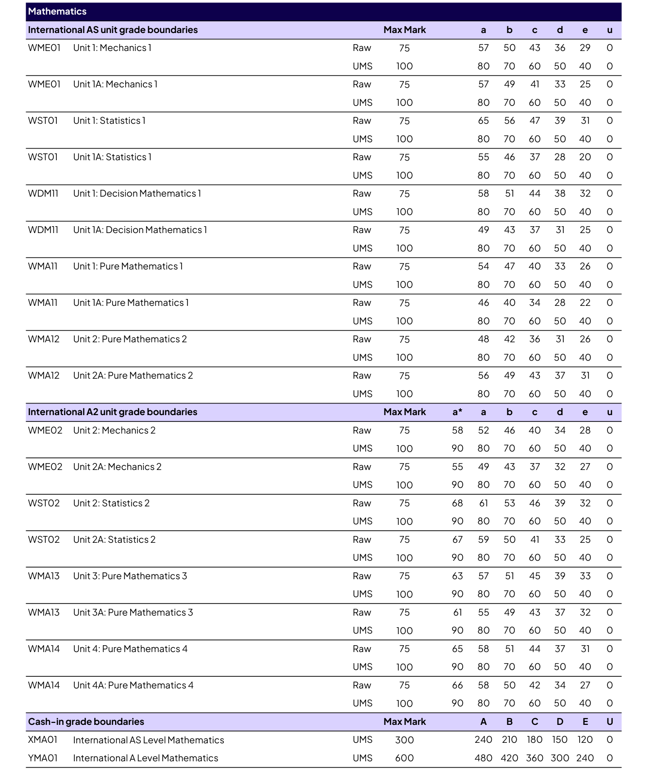
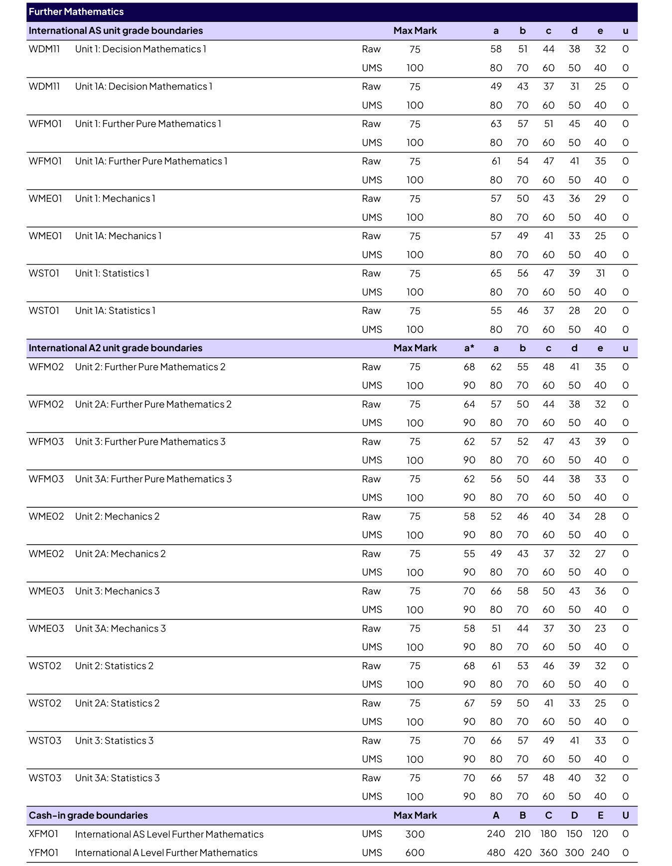
📍 2026年1月考季
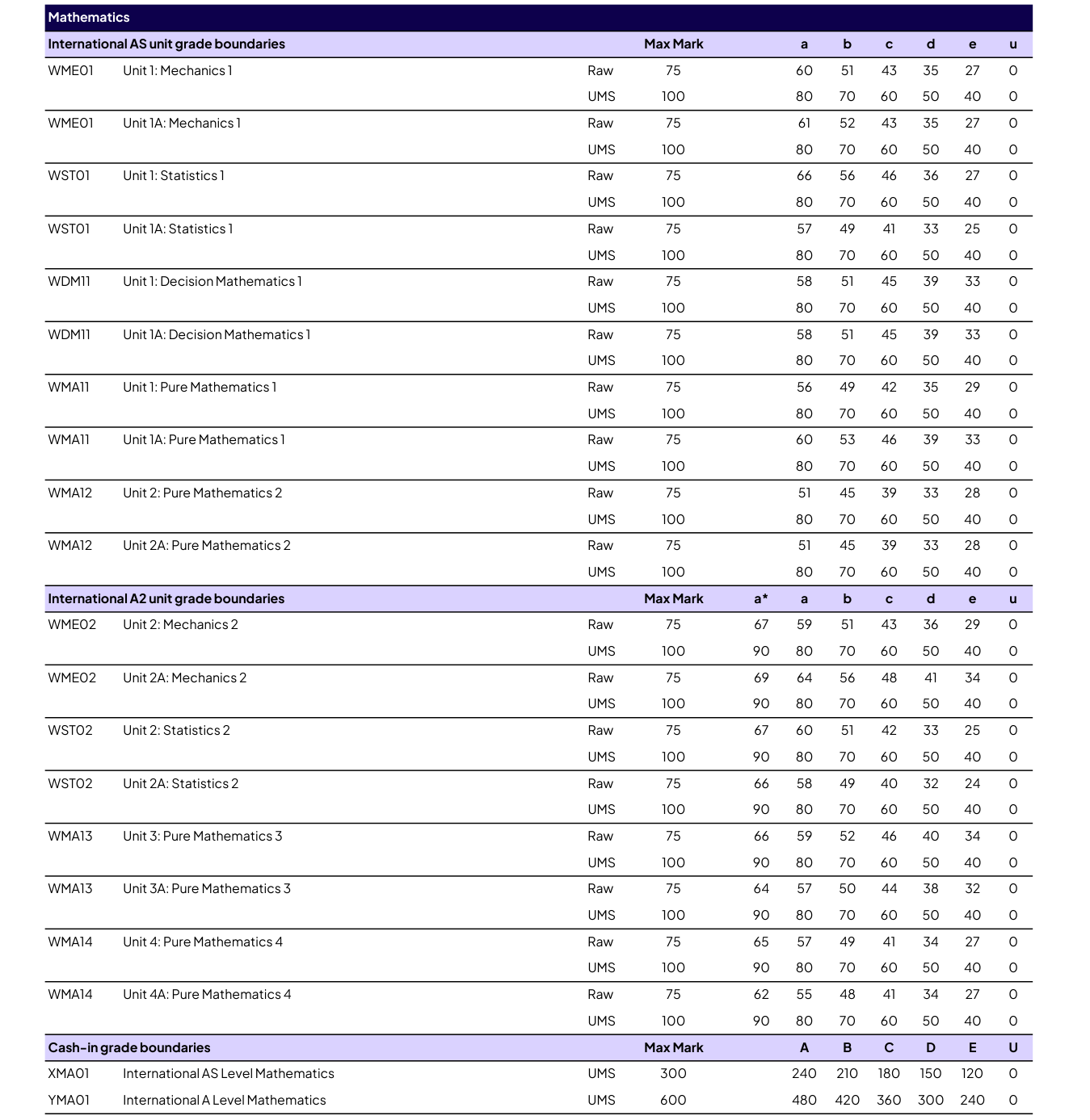
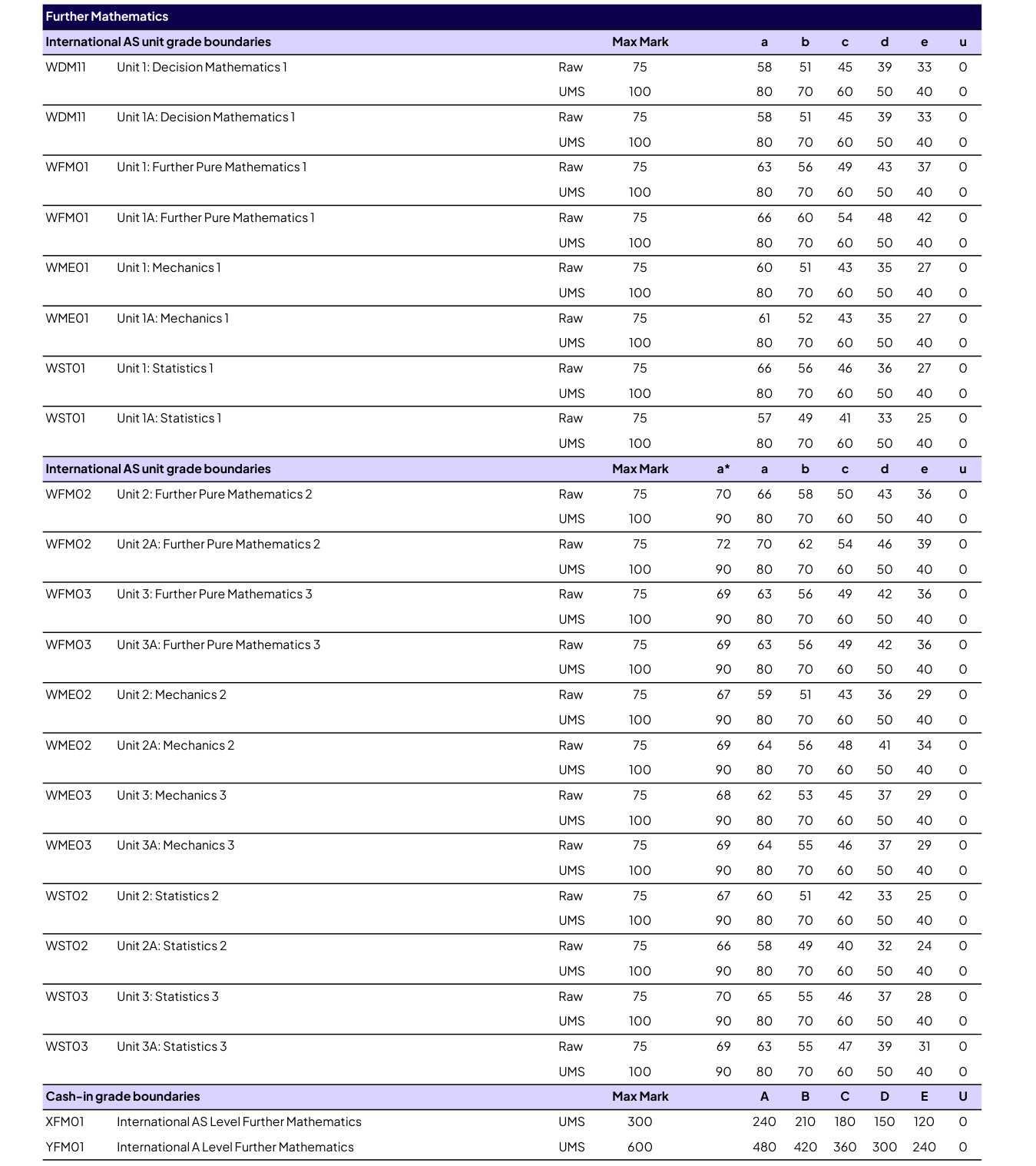
📍 2025年10月考季
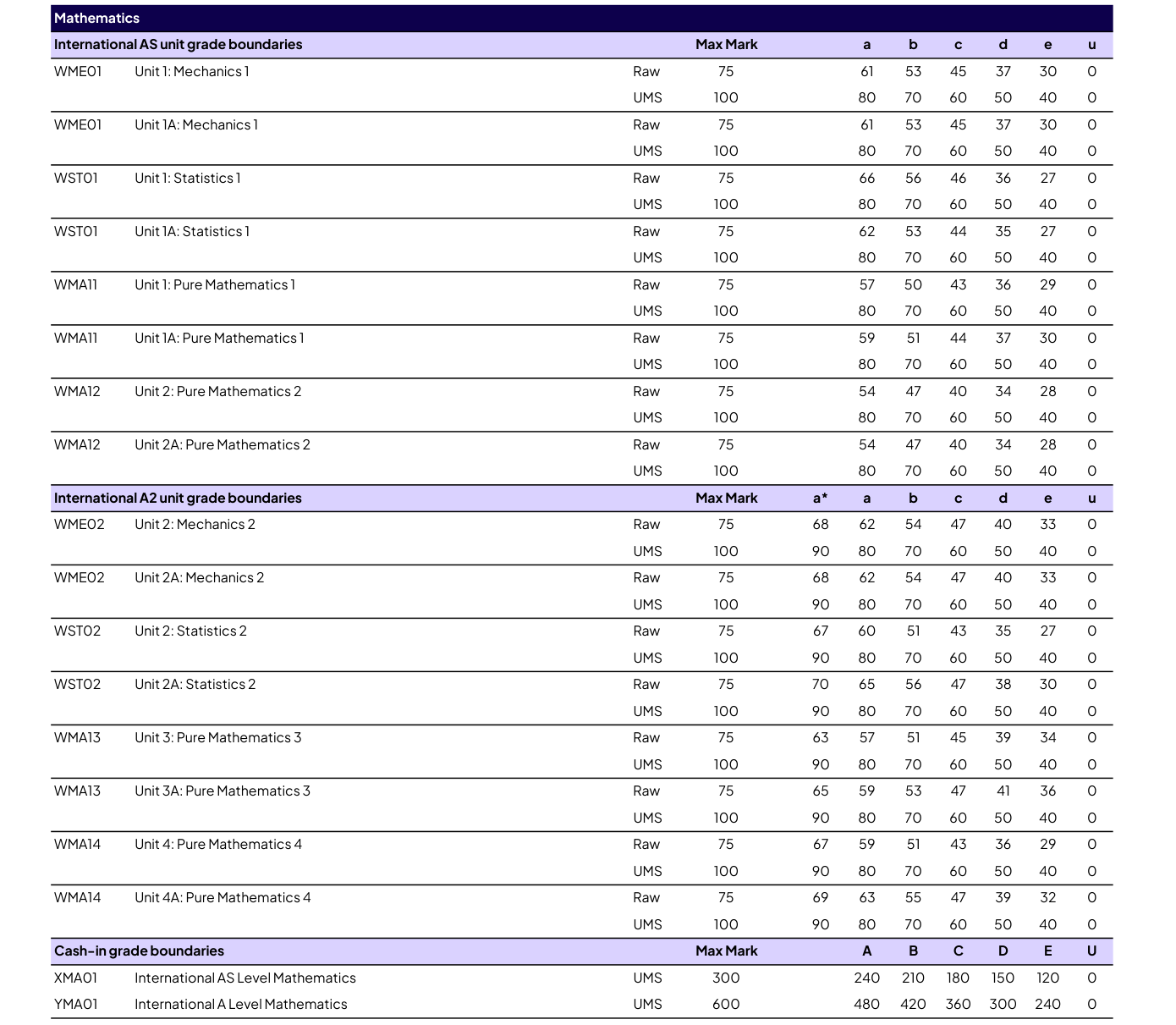
截图来源:qualifications.pearson.com 官方「Grade boundaries — International A Level」文件(2026 年 6 月 / 2026 年 1 月 / 2025 年 10 月考季)。2025 年 10 月考季官方文件未含进阶数学段落(该考季未开放相应单元)。
📝 S1 分类真题 Categorised Past Papers
Edexcel IAL WST01 (S1) 2019–2026 共 23 卷 / 156 题(含 01a 区域变体), 按官方规格 6 个章节、25 个知识点双语分类。点开任一知识点即可看到对应年份的真题; 每题附「题目 Question」与「详解 Mark Scheme」两个链接,均为所在完整试卷页原版(PDF 整页,不裁剪)。
同一知识点可能出现在多个章节之下(各章只列属于该章的题)。
1 · 统计建模 Statistical modelling (1 题)
统计模型与假设 Statistical models and assumptions (1 题)
| 试卷 Session | 题号 | 分值 | 链接 Links |
|---|---|---|---|
| 2024 Oct | Q5 | 8 | 题目 Question · 详解 Mark Scheme |
2 · 数据的表示与汇总 Representation and summary of data (36 题)
数据图表 Diagrams (stem-and-leaf, box plots, histograms) (18 题)
| 试卷 Session | 题号 | 分值 | 链接 Links |
|---|---|---|---|
| 2019 Jan | Q4 | 13 | 题目 Question · 详解 Mark Scheme |
| 2019 Jun | Q2 | 13 | 题目 Question · 详解 Mark Scheme |
| 2019 Oct | Q2 | 13 | 题目 Question · 详解 Mark Scheme |
| 2020 Jan | Q4 | 14 | 题目 Question · 详解 Mark Scheme |
| 2020 Oct | Q4 | 14 | 题目 Question · 详解 Mark Scheme |
| 2021 Jun | Q3 | 14 | 题目 Question · 详解 Mark Scheme |
| 2022 Jan | Q3 | 10 | 题目 Question · 详解 Mark Scheme |
| 2022 Jun | Q1 | 11 | 题目 Question · 详解 Mark Scheme |
| 2023 Jan | Q1 | 10 | 题目 Question · 详解 Mark Scheme |
| 2023 Jun | Q1 | 8 | 题目 Question · 详解 Mark Scheme |
| 2024 Jan | Q1 | 8 | 题目 Question · 详解 Mark Scheme |
| 2024 Jun | Q1 | 13 | 题目 Question · 详解 Mark Scheme |
| 2024 Jun | Q3 | 14 | 题目 Question · 详解 Mark Scheme |
| 2025 Jan | Q2 | 12 | 题目 Question · 详解 Mark Scheme |
| 2025 Jan | Q7 | 8 | 题目 Question · 详解 Mark Scheme |
| 2025 Oct 01A | Q3 | 11 | 题目 Question · 详解 Mark Scheme |
| 2026 Jan 01A | Q2 | 9 | 题目 Question · 详解 Mark Scheme |
| 2026 Jun 01A | Q2 | 13 | 题目 Question · 详解 Mark Scheme |
编码 Coding Coding (8 题)
| 试卷 Session | 题号 | 分值 | 链接 Links |
|---|---|---|---|
| 2019 Jun | Q1 | 9 | 题目 Question · 详解 Mark Scheme |
| 2022 Jun | Q3 | 14 | 题目 Question · 详解 Mark Scheme |
| 2022 Oct | Q3 | 10 | 题目 Question · 详解 Mark Scheme |
| 2023 Jun | Q3 | 9 | 题目 Question · 详解 Mark Scheme |
| 2024 Jan | Q2 | 12 | 题目 Question · 详解 Mark Scheme |
| 2024 Jan | Q4 | 12 | 题目 Question · 详解 Mark Scheme |
| 2024 Jun | Q3 | 14 | 题目 Question · 详解 Mark Scheme |
| 2025 Oct | Q5 | 10 | 题目 Question · 详解 Mark Scheme |
位置度量 Measures of location (mean, median, mode) (1 题)
| 试卷 Session | 题号 | 分值 | 链接 Links |
|---|---|---|---|
| 2019 Jun | Q1 | 9 | 题目 Question · 详解 Mark Scheme |
离散度量 Measures of dispersion (variance, SD, IQR) (2 题)
| 试卷 Session | 题号 | 分值 | 链接 Links |
|---|---|---|---|
| 2025 Jun | Q2 | 7 | 题目 Question · 详解 Mark Scheme |
| 2025 Oct 01A | Q7 | 9 | 题目 Question · 详解 Mark Scheme |
四分位数与百分位数 Quartiles and percentiles (7 题)
| 试卷 Session | 题号 | 分值 | 链接 Links |
|---|---|---|---|
| 2023 Oct | Q2 | 13 | 题目 Question · 详解 Mark Scheme |
| 2024 Oct | Q1 | 10 | 题目 Question · 详解 Mark Scheme |
| 2025 Oct | Q2 | 11 | 题目 Question · 详解 Mark Scheme |
| 2025 Oct 01A | Q3 | 11 | 题目 Question · 详解 Mark Scheme |
| 2026 Jan | Q1 | 12 | 题目 Question · 详解 Mark Scheme |
| 2026 Jan 01A | Q2 | 9 | 题目 Question · 详解 Mark Scheme |
| 2026 Jun 01A | Q2 | 13 | 题目 Question · 详解 Mark Scheme |
离群值 Outliers (9 题)
| 试卷 Session | 题号 | 分值 | 链接 Links |
|---|---|---|---|
| 2019 Jun | Q2 | 13 | 题目 Question · 详解 Mark Scheme |
| 2020 Oct | Q4 | 14 | 题目 Question · 详解 Mark Scheme |
| 2022 Jan | Q3 | 10 | 题目 Question · 详解 Mark Scheme |
| 2022 Jun | Q1 | 11 | 题目 Question · 详解 Mark Scheme |
| 2023 Jun | Q3 | 9 | 题目 Question · 详解 Mark Scheme |
| 2023 Oct | Q2 | 13 | 题目 Question · 详解 Mark Scheme |
| 2024 Jun | Q1 | 13 | 题目 Question · 详解 Mark Scheme |
| 2025 Oct | Q2 | 11 | 题目 Question · 详解 Mark Scheme |
| 2026 Jan | Q1 | 12 | 题目 Question · 详解 Mark Scheme |
线性插值 Linear interpolation (10 题)
| 试卷 Session | 题号 | 分值 | 链接 Links |
|---|---|---|---|
| 2019 Jan | Q4 | 13 | 题目 Question · 详解 Mark Scheme |
| 2020 Jan | Q4 | 14 | 题目 Question · 详解 Mark Scheme |
| 2021 Jun | Q3 | 14 | 题目 Question · 详解 Mark Scheme |
| 2022 Oct | Q1 | 11 | 题目 Question · 详解 Mark Scheme |
| 2023 Jan | Q1 | 10 | 题目 Question · 详解 Mark Scheme |
| 2024 Jan | Q1 | 8 | 题目 Question · 详解 Mark Scheme |
| 2025 Jun | Q5 | 14 | 题目 Question · 详解 Mark Scheme |
| 2026 Jan 01A | Q5 | 13 | 题目 Question · 详解 Mark Scheme |
| 2026 Jun | Q3 | 10 | 题目 Question · 详解 Mark Scheme |
| 2026 Jun 01A | Q4 | 13 | 题目 Question · 详解 Mark Scheme |
频数分布与分组数据 Frequency distributions and grouped data (9 题)
| 试卷 Session | 题号 | 分值 | 链接 Links |
|---|---|---|---|
| 2019 Oct | Q2 | 13 | 题目 Question · 详解 Mark Scheme |
| 2022 Jun | Q3 | 14 | 题目 Question · 详解 Mark Scheme |
| 2022 Oct | Q1 | 11 | 题目 Question · 详解 Mark Scheme |
| 2023 Jun | Q1 | 8 | 题目 Question · 详解 Mark Scheme |
| 2025 Jun | Q5 | 14 | 题目 Question · 详解 Mark Scheme |
| 2025 Oct | Q5 | 10 | 题目 Question · 详解 Mark Scheme |
| 2026 Jan 01A | Q5 | 13 | 题目 Question · 详解 Mark Scheme |
| 2026 Jun | Q3 | 10 | 题目 Question · 详解 Mark Scheme |
| 2026 Jun 01A | Q4 | 13 | 题目 Question · 详解 Mark Scheme |
加权与组合数据集 Weighted and combined data sets (3 题)
| 试卷 Session | 题号 | 分值 | 链接 Links |
|---|---|---|---|
| 2022 Oct | Q3 | 10 | 题目 Question · 详解 Mark Scheme |
| 2025 Jan | Q2 | 12 | 题目 Question · 详解 Mark Scheme |
| 2025 Jun | Q2 | 7 | 题目 Question · 详解 Mark Scheme |
偏度与分布比较 Skewness and comparing distributions (2 题)
| 试卷 Session | 题号 | 分值 | 链接 Links |
|---|---|---|---|
| 2024 Oct | Q1 | 10 | 题目 Question · 详解 Mark Scheme |
| 2025 Oct 01A | Q7 | 9 | 题目 Question · 详解 Mark Scheme |
3 · 概率 Probability (35 题)
概率基础与维恩图 Probability basics and Venn diagrams (17 题)
| 试卷 Session | 题号 | 分值 | 链接 Links |
|---|---|---|---|
| 2019 Jan | Q1 | 9 | 题目 Question · 详解 Mark Scheme |
| 2019 Oct | Q5 | 12 | 题目 Question · 详解 Mark Scheme |
| 2020 Jan | Q2 | 12 | 题目 Question · 详解 Mark Scheme |
| 2021 Jun | Q2 | 12 | 题目 Question · 详解 Mark Scheme |
| 2022 Jan | Q1 | 11 | 题目 Question · 详解 Mark Scheme |
| 2022 Jun | Q4 | 11 | 题目 Question · 详解 Mark Scheme |
| 2022 Oct | Q6 | 11 | 题目 Question · 详解 Mark Scheme |
| 2023 Jan | Q4 | 13 | 题目 Question · 详解 Mark Scheme |
| 2023 Oct | Q3 | 12 | 题目 Question · 详解 Mark Scheme |
| 2024 Jun | Q6 | 13 | 题目 Question · 详解 Mark Scheme |
| 2024 Oct | Q3 | 8 | 题目 Question · 详解 Mark Scheme |
| 2025 Jan | Q4 | 9 | 题目 Question · 详解 Mark Scheme |
| 2025 Jun | Q4 | 4 | 题目 Question · 详解 Mark Scheme |
| 2025 Oct | Q6 | 9 | 题目 Question · 详解 Mark Scheme |
| 2025 Oct 01A | Q5 | 9 | 题目 Question · 详解 Mark Scheme |
| 2026 Jan | Q3 | 9 | 题目 Question · 详解 Mark Scheme |
| 2026 Jun | Q6 | 10 | 题目 Question · 详解 Mark Scheme |
条件概率 Conditional probability (24 题)
| 试卷 Session | 题号 | 分值 | 链接 Links |
|---|---|---|---|
| 2019 Jun | Q3 | 13 | 题目 Question · 详解 Mark Scheme |
| 2020 Oct | Q2 | 13 | 题目 Question · 详解 Mark Scheme |
| 2021 Jun | Q1 | 5 | 题目 Question · 详解 Mark Scheme |
| 2022 Jan | Q1 | 11 | 题目 Question · 详解 Mark Scheme |
| 2022 Oct | Q6 | 11 | 题目 Question · 详解 Mark Scheme |
| 2023 Jan | Q2 | 10 | 题目 Question · 详解 Mark Scheme |
| 2023 Jun | Q4 | 9 | 题目 Question · 详解 Mark Scheme |
| 2023 Jun | Q6 | 9 | 题目 Question · 详解 Mark Scheme |
| 2023 Oct | Q1 | 11 | 题目 Question · 详解 Mark Scheme |
| 2024 Jan | Q3 | 8 | 题目 Question · 详解 Mark Scheme |
| 2024 Jan | Q6 | 9 | 题目 Question · 详解 Mark Scheme |
| 2024 Oct | Q3 | 8 | 题目 Question · 详解 Mark Scheme |
| 2024 Oct | Q7 | 9 | 题目 Question · 详解 Mark Scheme |
| 2025 Jan | Q3 | 6 | 题目 Question · 详解 Mark Scheme |
| 2025 Jun | Q4 | 4 | 题目 Question · 详解 Mark Scheme |
| 2025 Jun | Q7 | 13 | 题目 Question · 详解 Mark Scheme |
| 2025 Oct | Q6 | 9 | 题目 Question · 详解 Mark Scheme |
| 2025 Oct | Q8 | 7 | 题目 Question · 详解 Mark Scheme |
| 2026 Jan | Q3 | 9 | 题目 Question · 详解 Mark Scheme |
| 2026 Jan | Q5 | 10 | 题目 Question · 详解 Mark Scheme |
| 2026 Jan 01A | Q7 | 12 | 题目 Question · 详解 Mark Scheme |
| 2026 Jun | Q2 | 8 | 题目 Question · 详解 Mark Scheme |
| 2026 Jun 01A | Q1 | 8 | 题目 Question · 详解 Mark Scheme |
| 2026 Jun 01A | Q5 | 9 | 题目 Question · 详解 Mark Scheme |
树图 Tree diagrams (14 题)
| 试卷 Session | 题号 | 分值 | 链接 Links |
|---|---|---|---|
| 2019 Jun | Q3 | 13 | 题目 Question · 详解 Mark Scheme |
| 2020 Oct | Q2 | 13 | 题目 Question · 详解 Mark Scheme |
| 2021 Jun | Q1 | 5 | 题目 Question · 详解 Mark Scheme |
| 2023 Jan | Q2 | 10 | 题目 Question · 详解 Mark Scheme |
| 2023 Jun | Q4 | 9 | 题目 Question · 详解 Mark Scheme |
| 2023 Oct | Q1 | 11 | 题目 Question · 详解 Mark Scheme |
| 2024 Jan | Q3 | 8 | 题目 Question · 详解 Mark Scheme |
| 2024 Oct | Q7 | 9 | 题目 Question · 详解 Mark Scheme |
| 2025 Jan | Q3 | 6 | 题目 Question · 详解 Mark Scheme |
| 2025 Jun | Q7 | 13 | 题目 Question · 详解 Mark Scheme |
| 2025 Oct | Q8 | 7 | 题目 Question · 详解 Mark Scheme |
| 2026 Jan | Q5 | 10 | 题目 Question · 详解 Mark Scheme |
| 2026 Jun | Q2 | 8 | 题目 Question · 详解 Mark Scheme |
| 2026 Jun 01A | Q1 | 8 | 题目 Question · 详解 Mark Scheme |
互斥与独立事件 Mutually exclusive and independent events (14 题)
| 试卷 Session | 题号 | 分值 | 链接 Links |
|---|---|---|---|
| 2019 Jan | Q1 | 9 | 题目 Question · 详解 Mark Scheme |
| 2019 Oct | Q5 | 12 | 题目 Question · 详解 Mark Scheme |
| 2020 Jan | Q2 | 12 | 题目 Question · 详解 Mark Scheme |
| 2021 Jun | Q2 | 12 | 题目 Question · 详解 Mark Scheme |
| 2022 Jun | Q4 | 11 | 题目 Question · 详解 Mark Scheme |
| 2023 Jan | Q4 | 13 | 题目 Question · 详解 Mark Scheme |
| 2023 Jun | Q6 | 9 | 题目 Question · 详解 Mark Scheme |
| 2023 Oct | Q3 | 12 | 题目 Question · 详解 Mark Scheme |
| 2024 Jan | Q6 | 9 | 题目 Question · 详解 Mark Scheme |
| 2024 Jun | Q6 | 13 | 题目 Question · 详解 Mark Scheme |
| 2025 Jan | Q4 | 9 | 题目 Question · 详解 Mark Scheme |
| 2026 Jan 01A | Q7 | 12 | 题目 Question · 详解 Mark Scheme |
| 2026 Jun | Q6 | 10 | 题目 Question · 详解 Mark Scheme |
| 2026 Jun 01A | Q5 | 9 | 题目 Question · 详解 Mark Scheme |
4 · 相关与回归 Correlation and regression (25 题)
散点图与相关系数 Scatter diagrams and correlation (PMCC) (19 题)
| 试卷 Session | 题号 | 分值 | 链接 Links |
|---|---|---|---|
| 2019 Jan | Q6 | 18 | 题目 Question · 详解 Mark Scheme |
| 2019 Jun | Q6 | 13 | 题目 Question · 详解 Mark Scheme |
| 2019 Oct | Q4 | 6 | 题目 Question · 详解 Mark Scheme |
| 2020 Jan | Q3 | 13 | 题目 Question · 详解 Mark Scheme |
| 2022 Jan | Q2 | 6 | 题目 Question · 详解 Mark Scheme |
| 2022 Jun | Q2 | 14 | 题目 Question · 详解 Mark Scheme |
| 2022 Oct | Q2 | 13 | 题目 Question · 详解 Mark Scheme |
| 2023 Jan | Q6 | 14 | 题目 Question · 详解 Mark Scheme |
| 2023 Jun | Q2 | 13 | 题目 Question · 详解 Mark Scheme |
| 2023 Oct | Q6 | 12 | 题目 Question · 详解 Mark Scheme |
| 2024 Jun | Q4 | 13 | 题目 Question · 详解 Mark Scheme |
| 2024 Oct | Q2 | 11 | 题目 Question · 详解 Mark Scheme |
| 2025 Jan | Q6 | 12 | 题目 Question · 详解 Mark Scheme |
| 2025 Jun | Q3 | 14 | 题目 Question · 详解 Mark Scheme |
| 2025 Oct | Q1 | 12 | 题目 Question · 详解 Mark Scheme |
| 2025 Oct 01A | Q1 | 12 | 题目 Question · 详解 Mark Scheme |
| 2026 Jan | Q2 | 12 | 题目 Question · 详解 Mark Scheme |
| 2026 Jan 01A | Q3 | 15 | 题目 Question · 详解 Mark Scheme |
| 2026 Jun | Q5 | 11 | 题目 Question · 详解 Mark Scheme |
回归线 Regression line (y on x) (22 题)
| 试卷 Session | 题号 | 分值 | 链接 Links |
|---|---|---|---|
| 2019 Jan | Q6 | 18 | 题目 Question · 详解 Mark Scheme |
| 2019 Jun | Q6 | 13 | 题目 Question · 详解 Mark Scheme |
| 2019 Oct | Q1 | 11 | 题目 Question · 详解 Mark Scheme |
| 2020 Jan | Q3 | 13 | 题目 Question · 详解 Mark Scheme |
| 2020 Oct | Q5 | 15 | 题目 Question · 详解 Mark Scheme |
| 2021 Jun | Q6 | 16 | 题目 Question · 详解 Mark Scheme |
| 2022 Jan | Q6 | 13 | 题目 Question · 详解 Mark Scheme |
| 2022 Jun | Q2 | 14 | 题目 Question · 详解 Mark Scheme |
| 2022 Oct | Q2 | 13 | 题目 Question · 详解 Mark Scheme |
| 2023 Jan | Q6 | 14 | 题目 Question · 详解 Mark Scheme |
| 2023 Jun | Q2 | 13 | 题目 Question · 详解 Mark Scheme |
| 2023 Oct | Q6 | 12 | 题目 Question · 详解 Mark Scheme |
| 2024 Jun | Q4 | 13 | 题目 Question · 详解 Mark Scheme |
| 2024 Oct | Q2 | 11 | 题目 Question · 详解 Mark Scheme |
| 2025 Jan | Q6 | 12 | 题目 Question · 详解 Mark Scheme |
| 2025 Jun | Q3 | 14 | 题目 Question · 详解 Mark Scheme |
| 2025 Oct | Q1 | 12 | 题目 Question · 详解 Mark Scheme |
| 2025 Oct 01A | Q1 | 12 | 题目 Question · 详解 Mark Scheme |
| 2026 Jan | Q2 | 12 | 题目 Question · 详解 Mark Scheme |
| 2026 Jan 01A | Q3 | 15 | 题目 Question · 详解 Mark Scheme |
| 2026 Jun | Q7 | 10 | 题目 Question · 详解 Mark Scheme |
| 2026 Jun 01A | Q7 | 8 | 题目 Question · 详解 Mark Scheme |
插值与外推 Interpolation and extrapolation (4 题)
| 试卷 Session | 题号 | 分值 | 链接 Links |
|---|---|---|---|
| 2020 Oct | Q5 | 15 | 题目 Question · 详解 Mark Scheme |
| 2021 Jun | Q6 | 16 | 题目 Question · 详解 Mark Scheme |
| 2022 Jan | Q6 | 13 | 题目 Question · 详解 Mark Scheme |
| 2026 Jun | Q7 | 10 | 题目 Question · 详解 Mark Scheme |
5 · 离散随机变量 Discrete random variables (33 题)
概率分布表 Probability distribution tables (11 题)
| 试卷 Session | 题号 | 分值 | 链接 Links |
|---|---|---|---|
| 2019 Jan | Q2 | 10 | 题目 Question · 详解 Mark Scheme |
| 2019 Jun | Q5 | 14 | 题目 Question · 详解 Mark Scheme |
| 2020 Jan | Q1 | 5 | 题目 Question · 详解 Mark Scheme |
| 2022 Jan | Q7 | 11 | 题目 Question · 详解 Mark Scheme |
| 2022 Jun | Q5 | 14 | 题目 Question · 详解 Mark Scheme |
| 2023 Jan | Q3 | 11 | 题目 Question · 详解 Mark Scheme |
| 2025 Jan | Q1 | 15 | 题目 Question · 详解 Mark Scheme |
| 2025 Oct | Q3 | 6 | 题目 Question · 详解 Mark Scheme |
| 2025 Oct | Q4 | 10 | 题目 Question · 详解 Mark Scheme |
| 2026 Jan | Q4 | 13 | 题目 Question · 详解 Mark Scheme |
| 2026 Jan 01A | Q1 | 6 | 题目 Question · 详解 Mark Scheme |
期望与方差 Expectation and variance (25 题)
线性变换 Linear functions E(aX+b), Var(aX+b) (15 题)
| 试卷 Session | 题号 | 分值 | 链接 Links |
|---|---|---|---|
| 2019 Jan | Q2 | 10 | 题目 Question · 详解 Mark Scheme |
| 2019 Oct | Q7 | 15 | 题目 Question · 详解 Mark Scheme |
| 2021 Jun | Q5 | 15 | 题目 Question · 详解 Mark Scheme |
| 2022 Jan | Q4 | 13 | 题目 Question · 详解 Mark Scheme |
| 2023 Jun | Q5 | 13 | 题目 Question · 详解 Mark Scheme |
| 2023 Oct | Q4 | 12 | 题目 Question · 详解 Mark Scheme |
| 2024 Jan | Q7 | 10 | 题目 Question · 详解 Mark Scheme |
| 2024 Jun | Q2 | 12 | 题目 Question · 详解 Mark Scheme |
| 2025 Jun | Q1 | 9 | 题目 Question · 详解 Mark Scheme |
| 2025 Oct | Q3 | 6 | 题目 Question · 详解 Mark Scheme |
| 2025 Oct 01A | Q6 | 13 | 题目 Question · 详解 Mark Scheme |
| 2026 Jan | Q4 | 13 | 题目 Question · 详解 Mark Scheme |
| 2026 Jan | Q6 | 10 | 题目 Question · 详解 Mark Scheme |
| 2026 Jun | Q4 | 11 | 题目 Question · 详解 Mark Scheme |
| 2026 Jun 01A | Q3 | 14 | 题目 Question · 详解 Mark Scheme |
分布的构造 Constructing distributions (10 题)
| 试卷 Session | 题号 | 分值 | 链接 Links |
|---|---|---|---|
| 2019 Jan | Q5 | 15 | 题目 Question · 详解 Mark Scheme |
| 2020 Jan | Q6 | 17 | 题目 Question · 详解 Mark Scheme |
| 2020 Oct | Q1 | 5 | 题目 Question · 详解 Mark Scheme |
| 2022 Jan | Q7 | 11 | 题目 Question · 详解 Mark Scheme |
| 2022 Oct | Q4 | 4 | 题目 Question · 详解 Mark Scheme |
| 2022 Oct | Q7 | 14 | 题目 Question · 详解 Mark Scheme |
| 2024 Jan | Q7 | 10 | 题目 Question · 详解 Mark Scheme |
| 2024 Oct | Q6 | 14 | 题目 Question · 详解 Mark Scheme |
| 2025 Oct 01A | Q2 | 10 | 题目 Question · 详解 Mark Scheme |
| 2026 Jan 01A | Q4 | 11 | 题目 Question · 详解 Mark Scheme |
6 · 正态分布 The Normal Distribution (26 题)
标准化与查表 Standardisation and tables (26 题)
反查 z 求参数 Inverse z: finding mu and sigma (22 题)
| 试卷 Session | 题号 | 分值 | 链接 Links |
|---|---|---|---|
| 2019 Jan | Q3 | 10 | 题目 Question · 详解 Mark Scheme |
| 2019 Oct | Q6 | 10 | 题目 Question · 详解 Mark Scheme |
| 2020 Oct | Q3 | 13 | 题目 Question · 详解 Mark Scheme |
| 2021 Jun | Q4 | 13 | 题目 Question · 详解 Mark Scheme |
| 2022 Jan | Q5 | 11 | 题目 Question · 详解 Mark Scheme |
| 2022 Jun | Q6 | 11 | 题目 Question · 详解 Mark Scheme |
| 2022 Oct | Q5 | 12 | 题目 Question · 详解 Mark Scheme |
| 2023 Jan | Q5 | 17 | 题目 Question · 详解 Mark Scheme |
| 2023 Jun | Q7 | 14 | 题目 Question · 详解 Mark Scheme |
| 2023 Oct | Q5 | 15 | 题目 Question · 详解 Mark Scheme |
| 2024 Jan | Q8 | 9 | 题目 Question · 详解 Mark Scheme |
| 2024 Jun | Q5 | 10 | 题目 Question · 详解 Mark Scheme |
| 2024 Oct | Q4 | 5 | 题目 Question · 详解 Mark Scheme |
| 2024 Oct | Q8 | 10 | 题目 Question · 详解 Mark Scheme |
| 2025 Jan | Q5 | 13 | 题目 Question · 详解 Mark Scheme |
| 2025 Jun | Q6 | 14 | 题目 Question · 详解 Mark Scheme |
| 2025 Oct | Q7 | 10 | 题目 Question · 详解 Mark Scheme |
| 2025 Oct 01A | Q4 | 11 | 题目 Question · 详解 Mark Scheme |
| 2026 Jan | Q7 | 9 | 题目 Question · 详解 Mark Scheme |
| 2026 Jan 01A | Q6 | 9 | 题目 Question · 详解 Mark Scheme |
| 2026 Jun | Q8 | 12 | 题目 Question · 详解 Mark Scheme |
| 2026 Jun 01A | Q6 | 10 | 题目 Question · 详解 Mark Scheme |
正态分布的应用 Normal distribution applications (3 题)
| 试卷 Session | 题号 | 分值 | 链接 Links |
|---|---|---|---|
| 2019 Jun | Q4 | 13 | 题目 Question · 详解 Mark Scheme |
| 2020 Jan | Q5 | 14 | 题目 Question · 详解 Mark Scheme |
| 2024 Jan | Q5 | 7 | 题目 Question · 详解 Mark Scheme |
真题版权归 Pearson Edexcel 所有,此处仅作教学练习用途。
同一考季只保留一条链接:QP(试卷)/ MS(评分表)优先用 Pearson 官方直链,官方未公开该考季时才回退到第三方镜像 PMT(physicsandmathstutor.com,链接带 <em>PMT</em> 小标签);MA(Model Answers 详解)仅 PMT 有,ER(Examiner Report 考官报告)仅官方有。
⚠️ October 2025 / January 2026 / June 2026 三个考季:官方材料已上传但锁在教师账号后(访问跳登录页),第三方也尚未收录——本站不提供这三个考季的链接,需要请登录 Pearson 官方 course materials 页或经所在 centre 获取。
同一次考试可能有多个版本(如 Unit 1 与 Unit 1A),另有少量“(Unused)”备用卷,以表中实际列为准。
📄 Statistics 1(WST01)· 历年真题与评分材料
| 考季 | 试卷 QP | 评分表 MS | 详解 MA | 考官报告 ER |
|---|---|---|---|---|
| January 2019 | QP PMT | MS PMT | MA PMT | – |
| June 2019 | QP PMT | MS PMT | MA PMT | – |
| June 2020 | QP PMT | MS PMT | – | – |
| January 2021 | QP PMT | MS PMT | – | – |
| June 2021 | QP PMT | MS PMT | – | – |
| October 2021 | QP PMT | MS | – | – |
| January 2022 | QP PMT | MS PMT | – | ER |
| June 2022 | QP | MS | – | ER |
| October 2022 | QP | MS | – | ER |
| January 2023 | QP | MS | – | ER |
| June 2023 | QP | MS | – | ER |
| October 2023 | QP | MS | – | ER |
| January 2024 | QP | MS | – | ER |
| June 2024 | QP | MS | – | ER |
| October 2024 | QP | MS | – | ER |
| January 2025 | QP | MS | – | ER |
| June 2025 | QP | MS | – | ER |
本单元索引页:PMT https://www.physicsandmathstutor.com/a-level-maths-papers/edexcel-maths-ial-papers/; Pearson 官方 Mathematics (2018) course materials(需教师账号的考季也在这里登录获取)。
QP = Question paper 试卷 · MS = Mark scheme 评分表 · MA = Model answers 详解 · ER = Examiner report 考官报告。 未带小标签的为 **Pearson 官方**直链;带 PMT 小标签的为第三方镜像(physicsandmathstutor.com)。 同一考季同一文档只保留一条链接,官方优先。全部链接 2026-10-15 逐条实测可下载。